 Improve this document
 Create an issue
 Edit on GitHub
This document is also available in PDF format and in other languages: español.

Colophon
Suggested citation
Chapman AD & Wieczorek JR (2020) Georeferencing Best Practices. Copenhagen: GBIF Secretariat. https://doi.org/10.15468/doc-gg7h-s853
Licence
The document Georeferencing Best Practices is licensed under Creative Commons Attribution-ShareAlike 4.0 Unported License.
Abstract
Georeferencing Best Practices provides guidelines to the best practices for georeferencing. Though targeted specifically at biological occurrence data, the concepts and methods presented here may be just as useful in other disciplines.
Document control
v1.2.1, 10 July 2025
Originally based on an earlier publication, Chapman AD & Wieczorek JR (2006) Guide to Best Practices for Georeferencing. Copenhagen: GBIF Secretariat. https://doi.org/10.15468/doc-2zpf-zf42
Disclaimer
The information in this book represents the professional opinion of the authors, and does not necessarily represent the views of the publisher. While the authors and the publisher have attempted to make this book as accurate and as thorough as possible, the information contained herein is provided on an "As Is" basis, and without any warranties with respect to its accuracy or completeness. The authors and the publisher shall have no liability to any person or entity for any loss or damage caused by using the information provided in this book.
Where there are differences in interpretation between this document and translated versions in languages other than English, the English version remains the original and definitive version.
1. Introduction
| A Location that is poorly georeferenced obscures the information upon which a georeference should be based, potentially making the originally provided information irrecoverable. The resulting georeferences can be misleading to users and lead to errors in research outputs. Thus, an important take-home message is, "To georeference poorly is worse than not to georeference at all." |
Throughout this document we make use of terminology for which the specific meaning has great importance for overall understanding, especially for terms that might differ from, or vary in common usage. We mark these key words like this, with a link to the glossary, to call attention to the specific meaning and avoid potential confusion. All terms so marked are defined in the Glossary.
This publication provides guidelines to the best practice for georeferencing. Though it is targeted specifically at biological occurrence data, the concepts and methods presented here can be applied in other disciplines where spatial interpretation of location is of interest. This document builds on the original Guide to Best Practices for Georeferencing (Chapman & Wieczorek 2006), which was one of the outputs from the BioGeomancer project (Guralnick et al. 2006). Several earlier projects and organizations (e.g. MaNIS, MaPSTeDI, INRAM, GEOLocate, NatureServe, CRIA, ERIN, CONABIO) had previously developed guidelines and tools for georeferencing, and these provided a good starting point for such a document. A detailed history of the organizations involved in the development of BioGeomancer and of the original Guide was given in that source. Throughout this document we reference tools and methodologies developed by those organizations and we acknowledge the valuable work by those organizations in their development. This document attempts to bring best practices up to date with terms, technologies, and georeferencing recommendations that have been developed and refined since the original document was published.
This document is designed so that institutions with georeferencing commitments can extract those portions that apply to their own requirements and priorities, and adapt them if necessary where those practices vary from, or elaborate on, the ones given here. Derived works should be made publicly accessible and the derived georeferencing protocol should be cited in the metadata of any georeferenced records that were produced by it. Citing a published protocol when your own methods differ would violate the best practice principle of replicability, described in §1.5. An example of a citable protocol is the Georeferencing Quick Reference Guide (Zermoglio et al. 2020). This document should not be cited as a georeferencing protocol.
This version is a complete revision with many new and updated references. The major changes and additions in this edition include:
-
Redefined the term extent to conform with general English and common technical usage to mean a distance, area or volume within defined boundaries and added the term radial to cover the sense of the term "extent" in previous documents (Wieczorek 2001, Wieczorek et al. 2004, Chapman & Wieczorek 2006, Wieczorek et al. 2012a, Wieczorek & Bloom 2015).
-
Introduced the concept of the corrected center to replace geographic center wherever that was used in the past. This is an important change because the geographic center did not necessarily yield the correct minimum uncertainty due to the extent of a feature, the corrected center does.
-
Expanded the sections on elevation and updated them to provide the most recent information on recording elevation and of determining uncertainty due to accuracy of GPSs and DEMs.
-
Expanded information on GPS satellites to include information on the other GNSS satellite systems.
-
Added information on the use of smartphones and cameras to record GPS locations and elevations.
-
Elaborated on the shape georeferencing method, including steps to refine the point-radius georeferencing method.
-
Expanded the explanations to include ecological, marine and other data collected in transects, along irregular paths, in polygons, or on grids.
-
Added information on determining georeferences for subterranean locations such as caves, tunnels and mine sites.
-
Added information on bathymetry and underwater depths.
-
Integrated this document with the companion documents Georeferencing Quick Reference Guide (Zermoglio et al. 2020) and Georeferencing Calculator Manual (Bloom et al. 2020).
1.1. Objectives
This document aims to provide current best practice for using the point-radius, bounding box, and shape georeferencing methods, whether for new records in the field or for retrospective georeferencing of historic and un-georeferenced locations. We hope that the reader will come away from this document with, if nothing else, a good appreciation of the following essential principles:
-
No matter how specific a location might seem, every location has an associated uncertainty, and this uncertainty determines the conditions under which the spatial interpretation of the location can be used. Based on this, coordinates without a carefully determined uncertainty should not be considered a georeference, they should be considered coordinates whose meaning is not clear.
-
Interpretations of locations are fraught with a wide variety of sources of uncertainty, and these are not always trivial to aggregate into an overall uncertainty.
-
The best locality description is one that is specific, concise, complete, and unambiguous; the more detailed the description, the better the chance of getting a georeference that is reproducible and that minimizes the uncertainty.
-
Coordinate precision is not the same as coordinate uncertainty, it is just one of many factors contributing to the overall uncertainty.
-
Users of georeferences should take into account the uncertainty (or lack of its documentation) when choosing data for analyses, as without that information, analyses may be skewed and results biased or altogether wrong.
-
Coordinates alone can not generally be checked for consistency; a locality description provides a confirmation that coordinates are correct.
-
Coordinates alone do not unambiguously define a location, because:
-
coordinates require a coordinate reference system to anchor the coordinates in relation to the Earth
-
no location is a point; even the most specific locations have an extent
-
any device that provides coordinates has an associated uncertainty
Conclusion: coordinates alone do not constitute a georeference.
-
-
Geometries are great as georeferences, if you can deal with them; if not, the point-radius is surprisingly powerful, because using a Geographic Information System (GIS), it can be intersected with other spatial layers to get geometries (shapes).
1.2. Target Audience
This work is designed for those who need, or want to know why the best practices are what they are, in detail. This document is also for individuals or organizations faced with planning a georeferencing project by providing a series of questions that suggests particular subsets of the best practices to follow.
For those who just need to know how to put these practices into action while georeferencing, the Georeferencing Quick Reference Guide is the most suitable document to have at hand. The Quick Reference Guide refers to details in this document as needed and accompanies the Georeferencing Calculator, which is a tool to calculate coordinates and uncertainty following the methods described in this document.
Above all, this document will help data end users to understand the implications of trying to use records that have not undergone georeferencing best practices and the value of those that have.
1.3. Scope
This document is one of three that cover recommended requirements and methods to georeference locations. It is meant to cover the theoretical aspects (how to, and why) of spatially enabling information about the location of biodiversity-related phenomena, including special consideration for ecological and marine data. It also covers approaches to large-scale and collaborative georeferencing projects.
These documents DO NOT provide guidance on georectifying images or geocoding street addresses.
The accompanying Georeferencing Quick Reference Guide provides a practical how-to guide for putting the theory into practice, especially for the point-radius georeferencing method. The Quick Reference Guide relies on this document for background, definitions, more detailed explanations, while it describes exactly how to deal with a wide variety of specific cases (see §3.4.8).
The Georeferencing Calculator is a browser-based JavaScript application that aids in georeferencing descriptive localities and provides methods to help obtain geographic coordinates and uncertainties for locations (see §3.4.9).
1.4. Constraints
Constraints to using this document may arise because of:
-
Specimens with labels that are hard to read or decipher.
-
Records that don’t contain sufficient information.
-
Records that contain conflicting information.
-
Historic localities that are hard to find on current maps.
-
Locality names that have changed through time.
-
Marine locations from old ships' logs.
-
Lack of information on datums and/or coordinate reference systems.
-
Data Management Systems that don’t allow for recording or storage of the required georeferencing information.
-
Poor or no internet facilities.
-
Lack of access to suitable resources (maps, reliable gazetteers, etc.).
-
Lack of institutional/supervisor support.
-
Lack of training.
1.5. Principles of Best Practice
The following are principles of best practice that should be applied to georeferencing:
-
Accuracy – a measure of how well the data represent the truth, for example, how well is the true location of the target of an observation, collecting, or sampling event represented in a georeference. This includes considerations taken both at the moment when the location was recorded and when it was georeferenced. Note that careless lack of precision will have an adverse effect on accuracy (see §1.6).
-
Effectiveness – the likelihood that a work program achieves its desired objectives. For example, the percentage of records for which the coordinates and uncertainty can be accurately identified and calculated (see §6.8).
-
Efficiency – the relative effort needed to produce an acceptable output, including the effort to assemble and use external input data (e.g. gazetteers, collectors’ itineraries, etc.).
-
Reliability – the relative confidence in the repeatability or consistency with which information was produced and recorded. The reliability of sources and methods that can affect the accuracy of the results.
-
Accessibility – the relative ease with which users can find and use information in all of the senses supported by FAIR principles (Wilkinson et al. 2016) of data being Findable, Accessible, Interoperable, and Reusable.
-
Transparency – the relative clarity and completeness of the inputs and processes that produced a result. For example, the quality of the metadata and documentation of the methodology by which a georeference was obtained.
-
Timeliness – relates to the frequency of data collection, its reporting and updates. For example, how often are gazetteers updated, how long after georeferencing are the records made available to others, and how regularly are updates/corrections made following feedback.
-
Relevance – the relative pertinence and usability of the data to meet the needs of potential users in the sense of the principle of "fitness for use" (Chapman 2005a). Relevance is affected by the format of the output and whether the documentation and metadata are accessible to the user.
-
Replicability – the relative potential for a result to be reproduced. For example, a georeference following best practices would have sufficient documentation to be repeated using the same inputs and methods.
-
Adaptability – the potential for data to be reused under changing circumstances or for new purposes. For example, georeferences following best practices would have sufficient documentation to be used in analyses for which they were not originally intended.
In addition, an effective best practices document should:
-
Align the vision, mission, and strategic plans in an institution to its policies and procedures and gain the support of sponsors and/or top management.
-
Use a standard method of writing (writing format) to produce professional policies and procedures.
-
Satisfy industry standards.
-
Satisfy the scrutiny of management and external/internal auditors.
-
Adhere to relevant standards and biodiversity informatics practices.
1.6. Accuracy, Error, Bias, Precision, False Precision, and Uncertainty
There is often confusion around what is meant by accuracy, error, bias, precision, false precision, and uncertainty. In addition to the following paragraphs, refer to the definitions in the Glossary and Chapman 2005a. All of these concepts are relevant to measurements.
Accuracy, error, and bias all relate directly to estimates of true values. The closer a statement (e.g. a measurement) is to the true value, the more accurate it is. Error is a measure of accuracy–the difference between an estimated value and the true value. The more accurate an estimate, the smaller the error. Bias is a measurement of the average systematic error in a set of measurements. Bias often indicates a calibration or other systematic problem, and can be used to remove systematic errors from measurements, thus making them more accurate.
Because the true value is not known, but only estimated, the accuracy of the measured quantity is also unknown. Therefore, accuracy of coordinate information can only be estimated.
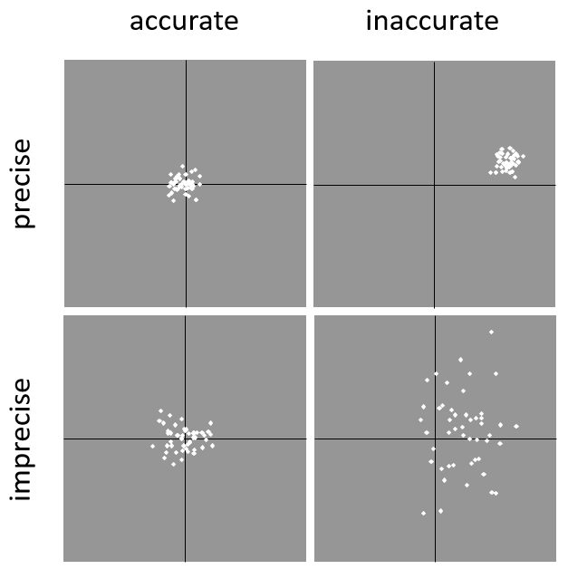
Whereas error is an estimate of the difference between a measured value and the truth, precision is a measurement of the consistency of repeated measurements to each other. Precision is not the same as accuracy (see Figure 1) because measurements can be consistently wrong (have the same error). Precise measurements of the same target will give similar results, accurate or not. We quantify precision as how specific a measurement should be to give consistent results. For example, a measuring device might give measurements to five decimal places (e.g. 3.14159), while repeated measurements of the same target with the same device are only consistent to four decimal places (e.g. 3.1416). We would say the precision is 0.0001 in the units of the measurement.
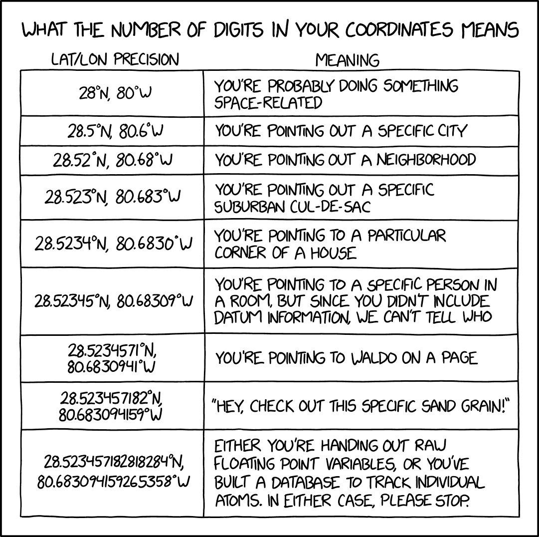
False precision refers to recorded values that have precision that is unwarranted by the original measurement. This is often an artefact of how data are stored, calculated, represented, or displayed. For example, a user interface might be designed to always display coordinates with five decimal places (e.g. 3.00000), demonstrating false precision for any coordinate that was not precise (e.g. 3°, a latitude given only to the nearest degree). Because false precision can be undetectable, the actual precision of a measurement is something that should be captured explicitly rather than inferred from the representation of a value. This is particularly true for coordinates, which can suffer from false precision as a result of a format transformation. For example, 3°20’ has a precision of one minute, equivalent to about 0.0166667 degrees, but when stored as decimal degrees where five decimal places are retained and displayed the value would be 3.33333, with a false precision of 0.00001 degrees. Also see Figure 2.
Like error, uncertainty is a measure of how different an unknown true value might be from a value given. In georeferencing, we use uncertainty to refer to the maximum distance from a center coordinate of a georeference to the furthest point where the true location might be–a combination of all the possible sources of error given as a distance.
1.7. Software and Online Tools
Software and tools come and go and are regularly updated, so rather than include a list in this document, we refer readers to georeferencing.org.
1.8. Conformance to Standards
Throughout this document, we have, where possible, recommended practices that conform to appropriate geographic information standards and standards for the transfer of biological and geographic information. These include standards developed by the Open Geospatial Consortium (OGC 2019), the Technical Committee for digital geographic information and geomatics (ISO/TC 211), and Biodiversity Information Standards (TDWG). Also, this document supports the FAIR principles of data management in recommending that well-georeferenced data are Findable, Accessible, Interoperable, and Reusable.
1.9. Persistent Identifiers (PIDs)
The use of Persistent Identifiers (PIDs) including Globally Unique Identifiers (GUIDs), Digital Object Identifiers (DOIs) etc. for uniquely identifying individual objects and other classes of data (such as collections, observations, images, and locations) are under discussion. It is important that any identifiers used are globally unique (applied to exactly one instance of an identifiable object), persistent, and resolvable (Page 2009, Richards 2010, Richards et al. 2011). As yet, very few institutions use PIDs for specimens, and even fewer for locations, however a recent paper by Nelson et al. 2018 makes a number of recommendations on minting, managing and sharing GUIDs for herbarium specimens. We recommend that once a stable system for assigning and using PIDs is implemented, it be used wherever practical, including for locations.
2. Elements for Describing a Location
In this section we discuss best practices for capturing and recording information so that it can be georeferenced and shared in the most productive and efficient way, following standard guidelines and methodologies. This will lead to improved consistency in recording, sharing, and use of data.
Collecting data in the field sets the stage for good georeferencing procedures (Museum of Vertebrate Zoology 2006). Many techniques now exist that can lead to well documented georeferenced locations. It is important, however, that the locations be recorded correctly in order to reduce the likelihood of error. We recommend that all new collecting events use a GPS for recording coordinates wherever possible, and that the GPS be set to a relevant datum or coordinate reference system (see §2.5). There are many issues that need to be considered when collecting data in the field and in this section we provide recommendations for best practice.
 MARINE. The principles as laid out in this document apply equally to marine data as to terrestrial and other data. For example, recording uncertainty for marine data is just as important as recording it for terrestrial systems. This is particularly important for legacy data, data from historic voyages, scientific expeditions, etc. There is also uncertainty for all recordings of a georeference - however small that may be with modern equipment. Note that there are a number of issues that apply only to marine information. We refer those working in marine systems to other parts of this document for issues such as depth, distance above surface, dealing with non-natural occurrences, recording extent of diving activities, etc. Where there are differences that specifically apply to marine locations, we will identify those with the icon.
 ECOLOGICAL DATA. Georeferencing ecological data, from surveys, trapping, species counts, etc. should be treated in a similar way to specimen and observation data. Often ecological data are recorded using a grid, or transect, and may have a starting locality and an ending locality as well as start time and end time. Where there are differences that specifically apply to ecological data, we will identify those with the icon.
 CAVES. Events in subterranean locations, such as in caves, tunnels and mines, pose special problems in determining the location. Where there are differences that specifically apply to these data, we will identify those with the icon.
2.1. The Importance of Good Locality Data
When recording data in the field, whether from a map or when using a GPS, it is important to record descriptive locality information as an independent validation of a georeference. The extent to which validation can occur depends on how well the locality description and its spatial counterpart describe the same place. The highest quality locality description is one contributing the least amount of uncertainty possible. This is equally important for retrospective georeferencing, where locality descriptions are given and georeferences are not, and for georeferencing in the field.
2.2. Localities
Provide a descriptive locality, even if you have coordinates. The locality should be as specific, succinct, unambiguous, complete, and as accurate as possible, leaving no room for multiple interpretations.
Features used as reference points should be stable, i.e. places (permanent landmarks, trig points, etc.) that will remain unchanged for a long time after the event is recorded. Do NOT use temporary features or waypoints as the key reference locality.
To facilitate the validation of a locality, use reference features that are easy to find on maps or in gazetteers. At all costs, avoid using vague terms such as "near" and "center of" or providing only an offset without a distance, such as "West of Jiuquan", or worse "W Jiuquan".
In any locality that contains a feature that can be confused with another feature of a different type, specify the feature type in parentheses following the feature name, for example, "Clear Lake (populated place)".
If recording locations on a path (road, river, etc.), it is important to also record whether the distances were measured along the actual path (e.g. ‘by road’) or as a direct line from the origin (e.g. ‘by air’).
| The most specific localities are those described by a) a distance and heading along a path from a nearby and well-defined intersection, or b) two cardinal offset distances from a single persistent nearby feature of small extent. |
| It is good practice not to use quotation marks ("") in locality descriptions as this can generate problems down the line if using open text files, spread sheets, etc. |
By describing a location in terms of a distance along a path, or by two orthogonal distances from a feature, one removes uncertainty due to imprecise headings, which, when the distances are great, can be the biggest contributing factor to overall uncertainty. Choosing a reference feature with small extent reduces the uncertainty due to the size of the reference feature, and by choosing a nearby reference feature, one reduces the potential for error in measuring the offset distances, especially along paths. The Museum of Vertebrate Zoology at the University of California, Berkeley has published a guide to recording good localities in the field that follows these principles. Following is an example locality from that document (copied with permission).
Locality: Modoc National Wildlife Refuge, 2.8 mi S and 1.2 mi E junction of Hwy. 299 and Hwy. 395 in Alturas, Modoc Co., Calif.
Lat/Long/Datum: 41.45063, −120.50763 (WGS84)
Elevation: 1330 ft
GPS Accuracy: 24 ft
Radial: 150 ft
References: Garmin Etrex Summit GPS for coordinates and accuracy, barometric altimeter for elevation.
When recording a location that does not have a feature that can be easily referenced, for example a dive location in the middle of the ocean (see entry point) or using some other marker that may only be recorded as a latitude and longitude, also record the provenance of the location (e.g. device or method used to determine the coordinates such as "transcription from ship’s log", etc.).
2.3. Extent of a Location
The extent of a location is the totality of the space it occupies. The extent is a simple way to alert the user that, for example, all of the specimens collected or observations made at the stated coordinates were actually within an area of up to 0.5 kilometers from that point. It can be quite helpful at times to include in your field notes a large-scale (highly detailed) map of the local vicinity for each locality, marking the area in which events actually occurred.
The extent may be a linear distance, an area or a volume represented by one or more buffered points (i.e. a point-radius), buffered lines (e.g. transects, stratigraphic sections), polygons, or other geometries in two or three dimensions (sphere, cube, etc.).
A location can be anchored to a position (as coordinates, potentially in combination with elevation, depth and distance above surface) within the extent. This may be the corner or center of a grid, the center of a polygon, the center of a circle, etc.
The geographic extent is the space occupied by the location when projected onto a 2D coordinate reference system in geographic coordinates (e.g. latitude and longitude in decimal degrees in WGS84 datum on Google Maps). The geographic radial is the line segment from the corrected center of the location to the furthest point on the boundary of the geographic extent of that location. This simplified representation may be convenient for many uses, as long as the references to the extent are not lost. With the coordinates alone, the nature of the extent and the variety of conditions found therein will be lost, thus sacrificing the utility of the spatial information about the location and the contexts in which the data can be used.
When recording observations, whether by people or from fixed recording instruments such as camera traps (Cadman & González-Talaván 2014), sound recorders, etc., the extent should include the effective field of view (for camera traps) or area of detectable signals covered by the sound recorders, etc. In these cases the most faithful representation of the location (the one that would allow for the least maximum uncertainty distance) should have the coordinates at the center of the extent of the field of detection, not at the position of the recording device or person. The true location may need to be calculated from the coordinates of the device using the radial and point-radius georeferencing method. If the position of the device or person is the only practical way to give the coordinates, then the radial for the location is the length of the furthest distance in the field of detection.
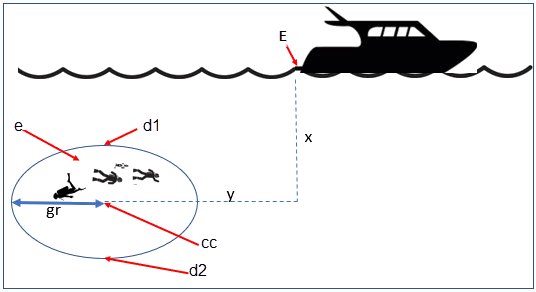
For diving activities, the coordinates are recorded as an entry point into the water and the locality is recorded with reference to that entry point. For example, "sampling was conducted in a rough sphere of 30 meters diameter, whose center was located 300 meters due west of the entry point at a depth between 50 and 100 meters". In these cases the radial must be big enough to encompass the position within the extent farthest from the entry point (see Figure 7).
2.3.1. Transects
For a location that is a transect, record both the start and end points of the line. This allows the orientation and direction of the transect to be preserved. If the events associated with the transect occur within a given maximum distance from the transect, it is better to represent the location as a polygon (see §2.3.3). If the events associated with the transect can be reasonably separated into their individual locations, it is better to do so, as these will be more specific than the transect as a whole. If that is done, however, ensure that you document that each individual location is part of a transect.
If the locality is recorded as the center of the transect and half the length of the transect is then used to describe uncertainty, information about the orientation of the transect is lost, and the description essentially becomes equivalent to a circle.
2.3.2. Paths
Not all linear-based locations are transects or straight lines. We use the term path to highlight this broader concept. Illustrative examples are: ad-hoc observations while walking along a trail, an inventory or count of species while travelling along a river, tracking an individual animal’s movements. Marine transects, tracks, tows, and trawls, are further examples. Paths should be described using shapes (see discussion under §3.3.4) as connected line segments (a polygonal chain), with the coordinates of the starting point followed by the coordinates of each segment beginning and finishing with the end point. One simple way to store and share these is through Well-Known Text (WKT) (ISO 2016, De Pooter et al. 2017, OBIS n.d., W.Appeltans, personal communication 15 Apr 2019).
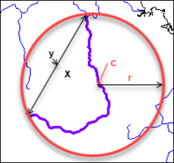
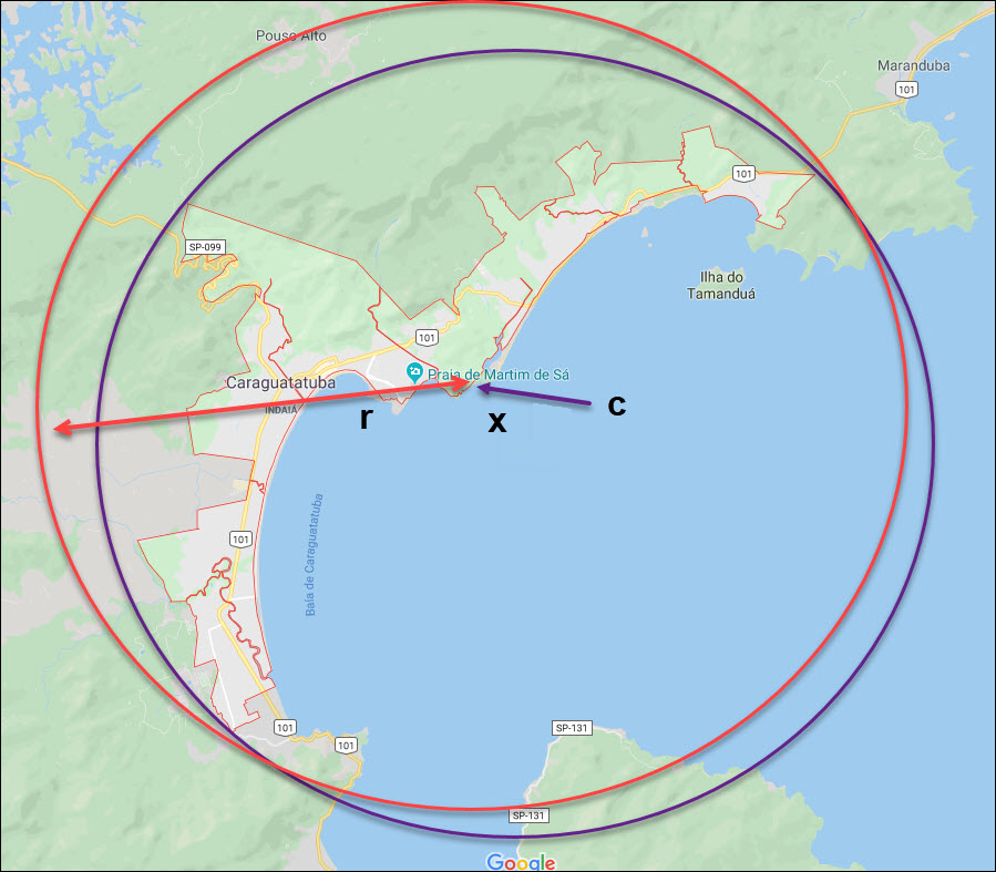
To determine the uncertainty of a described path using the point-radius georeferencing method, one needs to determine the corrected center – i.e. the point on the path that describes the smallest enclosing circle that includes the totality of the path ("c" on Figure 3). This is very seldom the same place as the center of a line joining the two ends of the path ("y" on Figure 3), nor the center of the extremes of latitude and longitude (the geographic center) of the path ("x" on Figure 3).
2.3.3. Polygons
When collecting or recording data from an area, for example, bird counts on a lake, a set of nesting or roosting sites on an offshore coral cay, or a buffered transect – the location is best recorded as a polygon. Polygons can be stored using the Darwin Core (Wieczorek et al. 2012b) field called dwc:footprintWKT, in which a geometry can be stored in the Well-Known Text format (ISO 2016). For the point-radius georeferencing method, if the polygon has a concave shape (for example a crescent), the center may not actually fall within the polygon (Figure 4). In that case, the corrected center on the boundary of the polygon is used for the coordinates of the location and the geographic radial is measured from that point to the furthest extremity of the polygon. Note that the circle based on the corrected center (red circle in Figure 4) will always be greater than the circle based on the geographic center (black circle in Figure 4).
Complex polygons, such as donuts, self-intersecting polygons and multipolygons create even more problems, in both documentation and storage.
2.3.4. Grids
Grids may be based on the lines of latitude and longitude, or they may be cells in a Cartesian coordinate system based on distances from a reference point. Usually grids are aligned North-South, and if not, their magnetic declination is essential to record. If the extent of a location is a grid cell, then the ideal way to record it would be the polygon consisting of the corners of the grid (i.e. a bounding box). The point-radius method can be used to capture the coordinates of the grid cell center and the distance from there to one of the furthest corners, but given that the geometries for grid cells are so simple, it is best to also capture them as polygons. Often grid cells (e.g. geographic grids) are described using the coordinates of the southwest corner of the grid. Using the southwest corner as the coordinates for a point-radius georeference is wasteful, since the geographic radial would be from there to the farthest corner, which would be twice as far as it would be if the center of the grid cell was used instead. In any case, the characteristics of the grid should be recorded with the locality information.
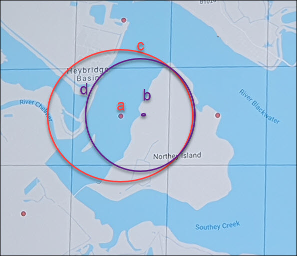
It is important when converting gridded data to geographic coordinates to also check the locality description. Locality information may allow you to refine the location as in Figure 5 where just having the grids without the locality information (i.e. "on Northey Island") would lead to the circle (c) with its center (a) at the center of the grid. Knowing that the record is on Northey Island, however, allows you to refine the location to the smaller circle (d) with its center at (b). Note that other criteria (such as a change of datum, map scale, etc.) may add to the uncertainty.
Township, Range and Section and Equivalents
Township, Range and Section (TRS) or Public Land Survey System (PLSS) is a grid-like way of dividing land into townships in the midwestern and western USA. Sections are usually one mile on each side and townships usually consist of 36 sections arranged in a grid with a specific numbering system. Not all townships are square, however, as there may be irregularities based on administrative boundaries, for example. For this reason, though these systems resemble grids, they are best treated as individual polygons. Similar subdivisions are used in other countries
Quarter Degree Grid Cells
Quarter Degree Grid Cells (QDGC) (Larsen et al. 2009, Larsen 2012) and their predecessor Quarter Degree Squares (QDS) have been used in many historical African biodiversity atlas projects and continue to be used for current South African biodiversity projects such as the Atlas of South African birds (Harrison et al. 1997). It has also been recommended as the method to use for generalizing sensitive biodiversity data in South Africa (SANBI 2016, Chapman 2020).
The QDGC method for recording grids follows an earlier system (QDS) that was developed for South Africa, and only worked in southern Africa, i.e. in the southern and eastern hemispheres. Larsen et al. (2009) provided an extension to the QDS standard that allowed the methodology to be used across the world in all hemispheres. To do this, they adapted the reference system to address locations independent of the hemisphere. This required the addition of characters delimiting north/south and east/west positions. An extra Zero was added to east/west references to pad to three characters. They changed the reference position for the grids to that which is closest to the Prime Meridian and the Equator (i.e., in northern hemisphere Africa, for example to the bottom left, while retaining the top left for southern Africa). The code is designated by:
-
A symbol denoting the eastern or western hemispheres (E or W).
-
The three-digit degree of longitude.
-
A symbol denoting the northern or southern hemisphere (N or S).
-
The two digit degree of latitude.
-
Each degree square is then divided into sixteen quarter-degree squares, each 15’ x 15’. These are given two additional letters as indicated. Thus in Figure 6, the green square is represented by the code E032S18CB.
The earlier Quarter Degree Square (QDS) methodology references this square as 3218CB. The QDS methodology is still commonly used in southern Africa, but is easily translatable to the QDGC system.

2.3.5. Three-Dimensional Shapes
Most terrestrial locations are recorded with reference to the terrestrial surface as geographic coordinates, sometimes with elevation. Some types of marine events such as dives and trawls, benefit from explicit description in three dimensions.
Diving events are commonly recorded using the geographic coordinates of the point on the surface where the diver entered the water, called entry point or point of entry. The underwater location should be recorded as a horizontal distance and direction along with water depth from that surface location (see Figure 7). Below the surface the diver may then begin a collection/observation exercise in three dimensions from that point including a horizontal component and a minimum and maximum water depth. These should all be recorded. The reference point should be the corrected center of the 3D-shape that includes the extent of the location. The geographic radial would be the distance from the corrected center of the 3D shape (the three dimensions projected perpendicularly onto the surface) to the furthest extremity of the projection of the 3D-shape in the horizontal plane (i.e. on the geographic boundary).
2.4. Coordinates
Whenever practical, provide the coordinates of the location where an event actually occurred (see §2.3) and accompany these with the coordinate reference system of the coordinate source (map or GPS). The two coordinate systems most commonly used by biologists are based on geographic coordinates (i.e. latitude and longitude) or Universal Transverse Mercator (UTM) (i.e. easting, northing and UTM zone).
A datum is an essential part of a coordinate reference system and provides the frame of reference. Without it the coordinates are ambiguous. When using both maps and GPS in the field, set the coordinate reference system or datum of the GPS or GNSS receiver to be the same as that of the map so that the GPS coordinates for a location will match those on the map. Be sure to record the coordinate reference system or datum used.
2.4.1. Geographic Coordinates
Geographic coordinates are a convenient way to define a location in a way that is not only more specific than is otherwise possible with a locality description, but also readily allows calculations to be made in a GIS. Geographic coordinates can be expressed in a number of different coordinate formats (decimal degrees, degrees minutes seconds, degrees decimal minutes), with decimal degrees being the most commonly used. Geographic coordinates in decimal degrees are convenient for georeferencing because this succinct format has global applicability and relies on just three attributes, one for latitude, one for longitude, and one for the geodetic datum or ellipsoid, which, together with the coordinate format, make up the coordinate reference system. By keeping the number of recorded attributes to a minimum, the chances for transcription errors are minimized (Wieczorek et al. 2004).
When capturing geographic coordinates, always include as many decimals of precision as given by the coordinate source. Coordinates in decimal degrees given to five decimal places are more precise than a measurement in degrees-minutes-seconds to the nearest second, and more precise than a measurement in degrees and decimal minutes given to three decimal places (see Table 3). Some new GPS/GNSS receivers now display data in decimal seconds to two decimal places, which corresponds to less than a meter everywhere on Earth. This doesn’t mean that the GPS reading is accurate at that scale, only that the coordinates as given do not contribute additional uncertainty.
| Decimal degrees are preferred when capturing coordinates from a GPS, however, where reference to maps is important, and where the GPS receiver allows, set the recorder to report in degrees, minutes, and decimal seconds. |
2.4.2. Universal Transverse Mercator (UTM) Coordinates
Universal Transverse Mercator (UTM) is a system for assigning distance-based coordinates using a Mercator projection from an idealized ellipsoid of the surface of the Earth onto a plane. In most applications of the UTM system, the Earth is divided into a series of six-degree wide longitudinal zones extending between 80°S and 84°N and numbered from 1-60 beginning with the zone at the Antimeridian (Snyder 1987). Because of the latitudinal limitation in extent, UTM coordinates are not usable in the extreme polar regions of the Earth. A map of UTM zones can be found at UTM Grid Zones of the World (Morton 2006).
UTM coordinates consist of a zone number, a hemisphere indicator (N or S), and easting and northing coordinate pairs separated by a space with 6 and 7 digits respectively, and all in the order given here. For example, for Big Ben in London (latitude 51.500721, longitude −0.124430), the UTM reference would be: 30N 699582 5709431.
Latitude bands are not officially part of UTM, but are used in the Military Grid Reference System (MGRS). They are used in many applications, including in Google Earth. Each zone is subdivided into 20 latitudinal bands, with letters used from South to North starting with "C" at 80°S to "X" (stretched by an extra 4 degrees) at 72°N (to 84°N) and omitting "O". All letters below "N" are in the southern hemisphere, "N" and above are in the northern hemisphere. When using latitudinal bands, "north" and "south" need to be spelled out to avoid confusion with the latitudinal bands of "N" and "S" respectively. Using the latitudinal band method, the coordinates for Big Ben would be: 30T 699582m east 5709431m north.
National and local grid systems derived from UTM, but which may be based on different ellipsoids and datums, are basically used in the same way as UTMs. For example, the Map Grid of Australia (MGA2020) uses UTM with the GRS80 ellipsoid and Geocentric Datum of Australia (GDA2020) (Geoscience Australia 2019b). An example of a location in MGA2020 is "MGA Zone 56, x: 301545 y: 7011991"
When recording a location, or databasing using UTM or equivalent coordinates, a zone should ALWAYS be included; otherwise the data are of little or no value when used outside that zone, and certainly of little use when combined with data from other zones. Zones are often not reported where a region (e.g. Tasmania) falls completely within one UTM zone. This is OK while the database remains regional, but is not suitable for exchange outside of the zone. When exporting data from databases like these, the region’s zone should be added prior to export or transfer. Better still, modify the database so that the zone remains with the coordinates.
Note that Darwin Core (Wieczorek et al. 2012b) supports UTM coordinates only in the verbatimCoordinates field. There are several tools to convert UTM coordinates to geographic coordinates, including Geographic/UTM Coordinate Converter (Taylor 2003)–see Georeferencing Tools. For details on georeferencing, see Coordinates – Universal Transverse Mercator (UTM) in Georeferencing Quick Reference Guide (Zermoglio et al. 2020).
| If using UTM coordinates, always record the UTM zone and the datum or coordinate reference system. |
2.5. Coordinate Reference System
Except under special circumstances (the poles, for example), coordinates without a coordinate reference system do not uniquely specify a location. Confusion about the coordinate reference system can result in positional errors of hundreds of meters. Positional shifts between what is recorded on some maps and WGS84, for example, may be between zero and 5359 m (Wieczorek 2019).
An unofficial (not governed by a standards body) set of EPSG (IOGP 2019) codes are often used (and misused) to designate datums. There are EPSG codes for a variety of entities (coordinate reference systems, areas of use, prime meridians, ellipsoids, etc.) in addition to datums, and the codes for these are often confused. For example, the code for the WGS84 coordinate reference system is EPSG:4326, while the code for the WGS84 datum is EPSG:6326 and the code for the WGS84 ellipsoid is EPSG:6422. The EPSG code has the advantage (when properly chosen) that it is explicit which type of entity it refers to, unlike the common name alone (e.g. "WGS84" alone could refer to the coordinate reference system, the datum, or the ellipsoid). Increasingly, GPS units are reporting coordinate reference systems as EPSG codes. Knowing the EPSG code for the coordinate reference system, one can determine the datum and ellipsoid for that system. It is thus recommended to record the EPSG code of the coordinate reference system if possible, otherwise, record the EPSG code of the datum if possible, otherwise, record the EPSG code of the ellipsoid. If none of these can be determined from the coordinate source, record "not recorded". This is important, as it determines the uncertainty due to an unknown datum (see §3.4.4) and has potentially drastic implications for the maximum uncertainty distance.
Sources of EPSG codes include epsg.io (Maptiler 2019), Apache 2019, EPSG Dataset v9.1 (IOGP 2019) and Geomatic Solutions 2018. When using a GPS, it is important to set and record the EPSG code of the coordinate reference system or datum. See discussion below under §3.4.
| If you are not basing your locality description on a map, set your GPS to report coordinates using the WGS84 datum or a recent local datum that approximates WGS84 (that may, for example, be legislated for your country) or the appropriate Coordinate Reference System (EPSG Code). Record the datum used in all your documentation. |
2.6. Using a GPS
GPS (Global Positioning System) technology uses triangulation between a GPS/GNSS receiver and GPS or GNSS satellites (Kaplan & Hegarty 2006, Van Sickle 2015, Novatel 2015). As the GNSS satellites are at known positions in space, and the GPS/GNSS receiver can determine the distances to the detected satellites, the position on earth can be calculated. A minimum of four GNSS satellites is required to determine a position on the earth’s surface (McElroy et al. 2007, Van Sickle 2015). This is not generally a limitation today, as one can often receive signals from a large number of satellites (up to 20 or more in some areas). Note, however, that just because your GNSS receiver is showing lots of satellites, it doesn’t mean that all are being used as the receiver’s ability to make use of additional satellites may be limited by its computational power (Novatel 2015). In the past, many GPS units only referenced the GPS (USA) satellites of which there are currently 31 (April 2019), but now many GPS/GNSS receivers are designed to access systems from other countries as well – such as GLONASS (Russia), BeiDou-2 (China), Galileo (Europe), NAVIC (India), and QZSS (Japan), making a total of about 112 currently accessible satellites (2019) with a further 23 to be brought into operation over the next few years. This number is increasing rapidly every year (Braun 2019). Prior to the removal of Selective Availability in May 2000, the accuracy of handheld GPS receivers in the field was around 100 meters or worse (McElroy et al. 2007, Leick 1995). The removal of this signal degradation technique has greatly improved the accuracy that can now generally be expected from GPS receivers (GPS.gov 2018).
To obtain the best possible accuracy, the GPS/GNSS receiver must be located in an area that is free from overhead obstructions and reflective surfaces and have a good field of view to a broad portion of the sky (for example, they do not work very well under a heavy forest canopy, although new satellite signal technology is improving the accuracy in these locations (Moore 2017)). The GPS/GNSS receiver must be able to record signals from at least four GNSS satellites in a suitable geometric arrangement. The best arrangement is to have "one satellite directly overhead and the other three equally spaced around the horizon" (McElroy et al. 2007). The GPS/GNSS receiver must also be set to an appropriate datum or coordinate reference system (CRS) for the area, and the datum or CRS that was used must be recorded (Chapman 2005a).
| Set your GPS to report locations in decimal degrees rather than make a conversion from another coordinate system as it is usually more precise (see Table 3), better and easier to store, and saves later transformations, which may introduce error. |
| An alternative where reference to maps is important, and where the GPS receiver allows it, is to set the recorder to report in degrees, minutes, and decimal seconds. |
2.6.1. Choosing a GPS or GNSS Receiver
One of the most important issues for consideration when choosing a GPS or GNSS receiver is the antenna. An antenna behaves both as a spatial and frequency filter, therefore, selecting the right antenna is critical for optimizing performance (Novatel 2015). One of the drawbacks with smartphones, for example, is the limited size of the GNSS antenna.
For information on issues to consider when selecting an appropriate GNSS antenna and/or GPS receiver, we refer you to Chapter 2 in Novatel 2015 and Chapter 10 in NLWRA 2008.
2.6.2. GPS Accuracy
Most GPS devices are able to report a theoretical horizontal accuracy based on local conditions at the time of reading (atmospheric conditions, reflectance, forest cover, etc.). For highly specific locations, it may be possible for the potential error in the GPS reading to be on the same order of magnitude as the extent of the location. In these cases, the GPS accuracy can make a non-trivial contribution to the overall uncertainty of a georeference.
The latest US Government commitment (US Deptartment of Defense and GPS Navstar 2008) is to broadcast the GPS signal in space "with a global average user range error (URE) of ≤7.8 m (25.6 ft.), with 95% probability". In reality, actual performance exceeds this, and in May 2016, the global average URE was ≤ 0.715 m (2.3 ft), 95% of the time (GPS.gov 2017). Though it does not mean that all receivers can obtain that accuracy, the accuracy of GPS receivers has improved and today most manufacturers of handheld GPS units promise errors of less than 5 meters in open areas when using four or more satellites. The need for four or more satellites to achieve these accuracies is because of the inaccuracies in the clocks of the GPS receivers as opposed to the much more accurate satellite clocks (Novatel 2015). The accuracy can be improved by averaging the results of multiple observations at a single location (McElroy et al. 2007), and some modern GPS receivers that include averaging algorithms can bring the accuracy to around three meters or less. According to GISGeography 2019a, “A well-designed GPS receiver can achieve a horizontal accuracy of 3 meters or better and vertical accuracy of 5 meters or better 95% of the time. Augmented GPS systems can provide sub-meter accuracy”. Another method to improve accuracy is to average over more than one GPS unit. Note that some GPS/GNSS receivers can record up to 20 decimal places of precision, but that doesn’t mean that is the accuracy of the unit.
2.6.3. Differential GNSS
The use of Differential GNSS (DGNSS) (incorporating Differential GPS (DGPS)) can improve accuracy considerably. DGNSS references a GNSS Base Station (usually a survey control point) at a known position to calibrate the receiving GNSS signal. The Base Station and handheld GNSS receiver reference the satellites’ positions at the same time and thus reduces error due to atmospheric conditions, as well as (to a lesser extent) satellite ephemeris (orbital location) and clock error (Novatel 2015). The handheld GNSS instrument applies the appropriate corrections to the determined position. Depending on the quality of the receivers used, one can expect an accuracy of <1 meter (USGS 2017). This accuracy decreases as the distance of the receiver from the Base Station increases. It is important to note that differential technology is not available in all areas – for example, in remote locations and remote islands, and the resulting accuracy may be less than expected. Again, averaging can further improve on these values (McElroy et al. 2007). It is important to note, however, that most DGNSS is post-processed. Records are stored in the GPS/GNSS unit and then post-processing software is run to improve the measurements once connected to a computer. Post processing is not as commonly used since the introduction of real-time DGNSS, such as the Satellite Based Augmentation System, see the next subsection below), and is now used mostly in surveying applications where high accuracy is required.
Marine horizontal position accuracy requirements are 2-5 meters (at a 95 percent confidence level) for safety of navigation in inland waters, 8-20 meters (95%) in harbor entrances and approaches, and horizontal position accuracies of 1-100 meters (95%) for resource exploration in coastal regions (Skone et al. 2004, Skone & Yousuf 2007). While DGNSS horizontal error bounds are specified as 10 meters (95%) studies have shown that under normal operating conditions accuracies fall well within this bound.
DGNSS accuracies are susceptible to severe degradation due to enhanced ionospheric effects associated with geomagnetic storms. Degradation can be in the order of 2-30 times in some areas and depending on the severity of the storm.
2.6.4. Satellite Based Augmentation System
Satellite Based Augmentation System (SBAS) is a collection of geosynchronous satellites originally developed for precision guidance of aircraft (Federal Aviation Administration 2020) and more recently to provide services for improving the accuracy, integrity and availability of basic GNSS signals (Novatel 2015). SBAS receivers are inexpensive examples of real-time differential correction. SBAS uses a network of ground-based reference stations to measure small variations in the GNSS satellite signals. Measurements from the reference stations are routed to master stations, which queue the received Deviation Correction (DC) and send the correction messages to geostationary satellites. Those satellites broadcast the correction messages back to Earth, where SBAS-enabled GPS/GNSS receivers use the corrections while computing their positions to improve accuracy. Separate corrections are calculated for ionospheric delay, satellite timing, and satellite orbits (ephemerides), which allows error corrections to be processed separately, if appropriate, by the user application.
Wide Area Augmentation System
The first Satellite Based Augmentation System (SBAS) system was Wide Area Augmentation System (WAAS) (Wide Area Augmentation System), which was originally developed to provide improved GPS accuracy and a certified level of integrity to the US aviation industry, such as to enable aircraft to conduct precision approaches to airports and for coastal navigation. It was later expanded to cover Canada and Mexico, providing a consistent coverage over North America.
European Geostationary Navigation Overlay Service
The European Geostationary Navigation Overlay Service (EGNOS) was developed as an augmentation system that improves the accuracy of positions derived from GPS signals and alerts users about the reliability of the GPS signals. Originally developed using three geostationary satellites covering European Union member states, EGNOS satellites have now also been placed over the eastern Atlantic Ocean, the Indian Ocean, and the African mid-continent.
Other SBAS Services
More recently, other Satellite Based Augmentation System (SBAS)s have been, or are in the process of being developed to cover other parts of the world, including MSAS (Japan and parts of Asia), GAGAN (India), SDCM (Russia), SNAS (China), AFI (Africa) and SACCSA (South and Central America) (ESA 2014). Australia and New Zealand are in the process of developing an SBAS system that will provide several decimeter accuracy across Australia and its marine areas, and one decimeter accuracy across New Zealand. The system will provide three services to users – an L1 system with sub one-meter horizontal accuracy for aviation purposes; a Dual-Frequency Multi-Constellation (DFMC) with sub one-meter accuracies; and a Precise Point Position (PPP) service (see §2.6.6) with accuracies of 10-15 cm (Guan 2019). Testing is scheduled for completion in July 2020 (Geoscience Australia 2019a).
Accuracy of SBAS Services
A study in 2016 determined that, over most of the USA, the accuracy of Wide Area Augmentation System (WAAS)-enabled, single-frequency GPS units was on the order of 1.9 meters at least 95 per cent of the time (FAA 2017). This may be lower in other parts of the world where Satellite Based Augmentation System (SBAS) stations are less common. Note that as most SBAS satellites are geostationary, blocked line of sight towards the equator (southwards in the northern hemisphere, or northwards in the Southern hemisphere) by buildings or heavy canopy cover will reduce the accuracy of SBAS correction, Also, during solar storms, the accuracy deteriorates by a factor of around 2.
Despite early indications that WAAS can significantly improve positional accuracy during the most severe period of geomagnetic storms, more recent studies in the USA and Canada have shown that the sparseness of WAAS stations and ionospheric grids do not lead to a significant improvement. (Skone & Yousuf 2007). With reference stations needing to have separations within 100 km, improvements are only likely in coastal and near coastal areas of North America and Europe in the foreseeable future.
2.6.5. Ground-based Augmentation System
Ground Based Augmentation Systems (GBAS), also known as Local Area Augmentation Systems (LAAS), provide differential corrections and satellite integrity monitoring in conjunction with VHF radio, to link to GNSS receivers. A GBAS consists of several GNSS antennas placed at known locations with a central control system and a VHF radio transmitter. GBAS is limited in its coverage and is used mainly for specific applications that require high levels of accuracy, availability and integrity, and is the system largely used for airport navigation systems.
2.6.6. Precise Point Positioning
Precise Point Positioning (PPP) depends on GNSS satellite clock and orbit corrections, generated from a network of global reference stations to remove GNSS system error and provide a high level (decimeter) of positional accuracy. Once the corrections are calculated, they are delivered to the end user via satellite or over the Internet.
Although similar to Satellite Based Augmentation System (SBAS) systems (see above), they generally provide a greater accuracy and have the advantage of providing a single, global reference stream as opposed to the regional nature of an SBAS system. Whereas SBAS is free, the use of PPP usually incurs a charge to access the corrections, so it is unlikely that the increased accuracy of PPP when compared to that of SBAS, will be a consideration for most biological applications.
2.6.7. Static GPS
Static GPS uses high precision instruments and specialist techniques and is generally employed only by surveyors. Surveys conducted in Australia using these techniques reported accuracies in the centimeter range. These techniques are unlikely to be extensively used with biological record collection due to the cost and general lack of requirement for such precision.
2.6.8. Dual and Multi-Frequency GPS
High-end dual and multi-frequency GPS/GNSS devices can bring accuracy to the centimeter level, and even mm level over the long-term (GPS.gov 2017). One of the ways this is done is by removing one of the largest contributors to overall satellite error - error due to the ionosphere (known as ionosphere error) (Novatel 2015).
2.6.9. Smartphones
GPS-enabled smartphones are typically accurate to within 4.9 m (16 ft.) under open sky, however, their accuracy worsens near buildings, bridges, and trees (GPS.gov 2017). A study by Tomaštik et al. 2017 found that the accuracy of smartphones in open areas was around 2-4 m. This decreased to 3-11 m in deciduous forest without leaves, and 3-20 m in deciduous forest with leaves. There are reports that the accuracy in some GPS-enabled smartphones will soon be improved to <1 meter (Moore 2017) and that accuracy in areas with restricted satellite view within cities will be improved drastically with inbuilt 3D smartphone apps and probabilistic shadow matching (Iland et al. 2018). In general, the GNSS chipsets in smartphones are quite good, and any loss of accuracy is usually due to the quality of the antenna, whose chief failing is due to their poor multipath suppression (Pirazzi et al. 2017). In some smartphones where good satellite coverage is unavailable (e.g. in cities and forests), the phone may introduce errors from bias in its internal clock (Pirazzi et al. 2017), leading to occasional large inaccuracies (Arturo Ariño Oct 2019, pers. comm.). Already the technology for better than 1 meter smartphone accuracy exists, but it is not available to the public due to the difficulty and cost of incorporating the technology into small smartphones (Braun 2019). The accuracies reported in most publications refer to studies in the USA, Europe, coastal Australia, India or Japan where good differential stations are plentiful. More studies are needed to test smartphone accuracies in remote locations and where differential stations are not available.
Smartphone GPS technology is changing rapidly and there is likely to be new and updated information even before this document is published.
2.6.10. GPS-enabled Cameras
We are not aware of the characteristics of the accuracy of GPS-enabled cameras, but we expect the accuracy to be similar to that of smartphones. One study, using three different cameras, showed variation between the three and the true location to be less than 3 m from the reported location (Doty 2017). Note that GPS-enabled cameras that are used for snorkeling and diving activities, will only give new GPS readings each time the camera is brought to the surface.
2.6.11. Diver-towed Underwater GPS Receivers
Over the years, a number of methods for tracking a diver underwater with a GPS have been tried with limited success. These included using a floating GPS receiver over the diver’s bubbles, and a GPS receiver on a raft towed by the diver that recorded intermittent readings to provide a dive transect (Schories & Niedzwiedz 2011). The most successful to date has been the use of a GPS antenna on a floating buoy that is attached by a cable to a diver-held GPS. These diver-towed underwater GPS/GNSS handheld receivers have been used for underwater monitoring studies for several years. Most dives using this method are at <20 meters as the signal deteriorates with cable length giving a maximum practical depth of 50 meters (Niedzwiedz & Schories 2013). One problem is cable drag, and it is almost impossible to determine the buoys offset exactly although Niedzwiedz & Schories 2013 provide formulae for attempting to do so. A study by the same authors (Schories & Niedzwiedz 2011) showed displacement of 2.3 m at a depth of 5 m, 3.2 m at 10-m depth, 4.6 m at 20-m depth, 5.5 m at 30-m depth, and 6.8 m at 40-m depth. These are in addition to GPS accuracy discussed under §2.6.2.
2.7. Elevation
Supplement the locality description with elevation information if this can be easily obtained. Elevation can be determined from a variety of sources while in the field, including altimeters, maps (both digital and paper), and GPS/GNSS receivers, each with associated uncertainties. Elevation can be estimated after the fact using Digital Elevation Models at the coordinates of the location. In any case, record the method used to determine the elevation.
Elevation markings can narrow down the area in which you place a point. More often than not, however, they seem to create inconsistency. While elevation should not be ignored, it is important to realize that elevation was often measured inaccurately and/or imprecisely, especially early in the 20th century. One of the best uses of elevation in a locality description is to pinpoint a location along a road or river in a topographically complex area, especially when the rest of the locality description is vague.
When adding elevation after the fact be aware that the elevation can vary considerably over a small area (especially in steep terrain) and that the uncertainty of the georeference must be taken into account when determining the elevation. Do not use the coordinates on their own.
2.7.1. Altimeters
A barometric altimeter uses changes in air pressure as a proxy for changes in elevation, and can be a reliable source of elevation if properly calibrated. Calibration requires that the elevation of the altimeter be set to a known starting elevation, which could be determined from a map, for example. Thereafter, as the altimeter goes higher or lower in elevation, it estimates the new elevation directly from the air pressure it experiences. Since weather conditions can change the air pressure independently of changes in elevation, it is important to re-calibrate the altimeter frequently, either by recording the elevation when you stop moving and resetting to that same elevation before starting out again, and/or by recalibrating to known elevations whenever you encounter them.
In theory it would be possible to use a barometric altimeter to determine elevations when in a subterranean location (cave, mine, etc.), but these situations are particularly prone to changes in air pressure independent from elevation changes (especially in caves with narrow openings), so recalibration would have to be particularly careful.
2.7.2. Maps
Elevation can be determined using the contours and spot height information from a suitable scale map of the area. In general, the uncertainty in the elevation when read from a map is half the contour interval.
For information on determining accuracy from a map, see §3.4.2.1.
2.7.3. GPS
Elevation accuracy as reported from a GPS has improved markedly in recent years, but elevation accuracy is not usually reported by GPS/GNSS receivers. As a general rule, for most non-Satellite Based Augmentation System (SBAS) or Wide Area Augmentation System (WAAS) enabled GPS/GNSS receivers, elevation error is approximately 2-3 times the horizontal error (USGS 2017). It is hard to find definitive information for smartphones, but it would appear that this same multiplier is a good rule for those as well. With WAAS-enabled GPS, the FAA reports that 95 per cent of the time vertical error is less than 4 meters (FAA 2019). However, the elevation reported on the GPS receiver or smartphone is not necessarily referring to mean sea level (MSL) as reported, but to the zero elevation of the ellipsoid of the datum – see discussion below.
Note that GPS elevation readings can represent one of at least two different values, depending on the method used by the GPS. Elevation reported can be the geometric height. This is the only value that GPS devices can actually measure, and is the height based on the ellipsoid of the datum. The elevation reported can also be the elevation above MSL, or orthometric height. These values are not directly measured by the GPS, but are calculated as the difference between the geometric height (measured) and the geoid height. The geoid height depends on the geoid and the datum you are trying to compare it against. Thus, to understand the potential difference between elevations based on MSL and those based on the geometric model, the geometric model (datum) must be known. To calculate the potential error using WGS84 datum at a given geographic location, use the Geoid Height Calculator (UNAVCO 2020). For further discussion about these methods, consult Eos Positioning Systems 2018. For a good explanation of the differences between the geoid and mean sea level, we refer you to GISGeography 2019b.
2.7.4. Vertical Datums
In 2022, the USA will release a new geometric reference frame and geopotential vertical datum that will replace existing USA geometric vertical datums. Similarly, over the next five years, Australia will move to a new generation height reference frame – the Australian Gravimetric Quasigeoid 2017 (AGQG 2017) (McCubbine et al. 2019). The new reference frames will rely primarily on Global Navigation Satellite Systems (GNSS), as well as on an updated gravimetric geoid model (National Geodetic Survey 2018). The new method of calculating vertical datums will improve vertical accuracies to around 1-2 cm, will provide more accurate GPS-determined elevations (Ellingson 2017), and will allow for dynamic updating. Other jurisdictions are likely to move to new methods of calculating vertical datums over time, meaning that within five years most users will be able to position themselves vertically using mobile Global Navigation Satellite Systems (GNSS) technology with sub-decimeter accuracy (Brown et al. 2019).
2.7.5. Digital Elevation Models
Digital Elevation Models (DEM) are based on elevations above mean sea level (or more recently, the geoid). The models are calculated using sophisticated interpolations and do not necessarily correspond to the actual surface elevation. DEM vertical accuracy is influenced by several factors such as grid size, slope, land cover, and geolocation (horizontal) error, as well as other biases due to the original DEM data collection (e.g. satellite imaging geometry) and/or production method (Mukherjee et al. 2013, Mouratidis & Ampatzidis 2019). Global DEMs such as the Advanced Spaceborne Thermal Emission and Reflection Radiometer (ASTER) Global DEM V2 (Meyer 2011) and the Shuttle Radar Topography Mission (SRTM) are based on 1 arc-second grids (about 30 m x 30 m) (Farr et al. 2007) and have an accuracy of better than 17 m and 10 m respectively (except for in steep terrain such as mountains, and areas with very smooth sandy surfaces with low signal to noise ratio, such as the Sahara Desert (Farr et al. 2007)). Local and regional DEMs may have a smaller grid size. For example, a 5 m grid in Australia, which has a vertical accuracy better than one meter, and even to 0.3 meter in some areas (Geoscience Australia 2018) or the European Digital Elevation Model, which has an accuracy of better than three meters (Mouratidis & Ampatzidis 2019). Note also that satellite image-based DEMs, being radar based, vary greatly over different land surfaces, forests, shrub or herbaceous vegetation, agricultural areas, bare areas, rocky surfaces, wetlands, and artificial surfaces such as cities. Also the radar can penetrate into areas of snow, ice, and sand (as in deserts) (Mouratidis & Ampatzidis 2019).
2.7.6. Smartphones
Some smartphones, whether they incorporate GPS capabilities or not, use apps that provide elevation values based on a DEM. With smartphone GPS apps, be aware that some devices and apps incorrectly record the method used. The uncertainty in elevation due to an unknown elevation source can be up to 100 meters. For example, the difference with datum WGS84 between the ellipsoid and geoid or mean sea level methods of reporting elevation is shown in Figure 8. Note also that these uncertainties are in addition to the uncertainties associated with the measurements themselves. The only true way of determining what your GPS receiver or smartphone is recording is to test it against a known elevation. Some preliminary studies by the authors show elevation accuracy from smartphones varies greatly in different areas of the world. In areas in the USA, Europe, Australia, Japan, etc. (where most published results are from) errors are generally within 10 meters or so, but in more remote areas (such as on a remote island in Fiji), errors in the order of ±60 meters are not uncommon. Using two different mobile applications at sea level at one location resulted in reported elevations from −24 m to +58.9 m. These studies are preliminary and more research is needed in different areas of the world.
2.7.7. GPS-enabled Digital Cameras
GPS-enabled digital cameras are like smartphones with respect to positional accuracy as they have similar sized in-board antennas. To conserve battery life, most GPS-enabled digital cameras have options to set positional update intervals. Depending on the camera, these can range from once every second to once every five minutes. The setting of this interval may have significant implications with respect to both coordinates and uncertainty.
Underwater digital cameras only update their position when the diver or snorkeler takes the camera above the surface long enough for the GPS to fix its position.
2.7.8. Google Earth
Using a large sample size (n>20,000) of GPS benchmarks in a variety of terrains in the United States, Wang et al. 2017 found that elevations in the Google Earth terrain model had a boundary of error interval at 95 per cent (BE95) of ±44 m, with worst-case scenarios around 200 m. The same study found that Google Earth terrain model had a BE95 of ±6 m along highways. Though we find no data for elsewhere in the world at this time, we recommend using the values extracted from the work of Wang et al. 2017 as estimates of elevational uncertainty when the source is the Google Earth terrain model. A second study using Google Earth to determine elevation in three regions of Egypt (El-Ashmawy 2016) on flat, medium, and steep terrains concluded that elevation data is more accurate in flat areas or areas with small height difference, with an accuracy of approximately 1.85 m (RMSE) and an error range of less than 3.72 m (and in some findings less than 1 m). Increasing the difference in height leads to decrease in the obtained accuracy with the RMSE rising to 5.69 m in steep terrain.
2.8. Headings
Compass directions (also known as headings) can be rather ambiguous. North, for example, might be any direction between northwest and northeast if more specific information is not provided. There are several ways to avoid ambiguity when recording headings. One way is to qualify the direction with "due" (e.g. "due north") if the heading warrants it. A second way to avoid ambiguity is to use two orthogonal headings in locality descriptions, making implicit that both components are "due". Finally, ambiguity can be reduced if headings are given in degrees from north (0° is north, 90° is east, 180° is south, and 270° is west).
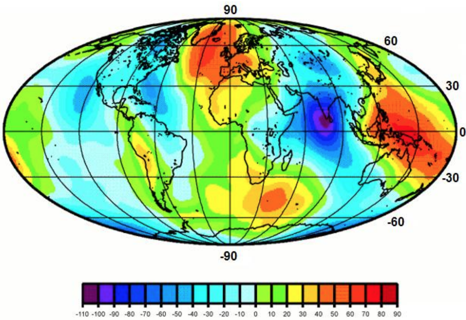
It is important to record headings based on True North (true heading) and not on Magnetic North (magnetic heading). The differences between True North and Magnetic North vary throughout the world, and in some places can vary greatly across a very small distance (NOAA 2019, NOAA/NCEI & CIRES 2019). For example, in an area about 250 km NW of Minneapolis in the United States, the anomalous magnetic declination (the difference between the declination caused by the Earth’s outer core and the declination at the surface) changes from 16.6° E to 12.0° W across a distance of just 6 km (Goulet 2001).
The differences between True North and Magnetic North also change over time (NOAA n.d.a). The National Oceanic and Atmospheric Administration (NOAA) has an online calculator that can calculate the anomalous or geomagnetic declination (adjustment needed to convert the magnetic reading to a reading based on True North) for any place on earth and at any point in time. If you need to make adjustments, we suggest that you use this calculator to determine the magnetic declination for the area in question. Otherwise determine your heading using a reliable map and always report your methods. Note that some smartphone apps will make that calculation for you, and allow you to set your app to record either Magnetic North or True North.
2.9. Offsets
An offset is a displacement from a reference point, named place, or other feature, and is generally accompanied by a direction (or heading, see §2.8). One of the best ways to describe a locality is with orthogonal offsets from a small, persistent, easy to locate feature (see §2.2). Using an offset at a very specific heading is a second option, though the uncertainty still grows with the offset distance. Offsets along a path are a third reasonable option for describing a locality, though they tend to be much harder to measure after the fact. Other locality types that use offsets (e.g. an offset direction without a distance, or an offset distance without a direction) tend to introduce excessive uncertainty and should be avoided.
2.9.1. Offset Distance Only
A locality consisting of an offset from a feature without a heading may arise as a result of an error when recording the locality in the field or through data entry. If the feature is small (such as a trig point) then the overall uncertainty will be largely due to the offset. With larger features (such as a town, or a lake), both the offset from, and the extent of the feature may contribute significantly to the overall uncertainty. The original collection catalogues or labels may contain information that can make the locality more specific. If not, a "Distance only" locality (e.g. "5 km from Lake Vättern, Sweden") might be envisioned as a band running around the reference feature at a distance given in the locality description. The problem is, we don’t know what was being used as the reference – some place in the lake, or some place on the edge — nor do we know if the offset was perpendicular to an edge or at some oblique angle to it. Because of these confounding factors, it is recommended to treat the locality as if it was a feature enlarged on all sides by the combination of all the sources of uncertainty (see Offset – Distance only in Georeferencing Quick Reference Guide (Zermoglio et al. 2020)).
2.9.2. Offset Direction Only
A locality with a heading from a feature, but with no distance (e.g. "East of Albuquerque"), is particularly ambiguous and very subjective to georeference. With no additional information to constrain the distance , there is no clear indication of how far one might have to go to reach the location – to the next nearest feature; the next nearest feature of equivalent size, to a place where there is a major change in biome (such as a coast), or just keep going?
Note that seldom is such locality information given alone. For example, the locality may have administrative geography information (e.g. ‘East of Albuquerque, Bernalillo County, New Mexico’). This gives you a stopping point (e.g. the county border), and should allow you to georeference the locality (see Offset – Heading only in Georeferencing Quick Reference Guide (Zermoglio et al. 2020)). In any case, it is highly recommended not to record locality descriptions in this way.
2.9.3. Offset at a Heading
A locality that contains an offset in a given direction to or from a feature is treated here as an "offset at a heading". There are several variations on such localities. One difficulty in determining a georeference for this type of locality description is knowing how the offset was determined – for example, by air, or along a path such as a road or river. Therefore, whenever a locality with an offset at a heading is described, be sure to be explicit about what is intended.
It is not uncommon for marine locality descriptions to use an azimuth – a heading toward a target feature, for example, "25° to Waipapa Point Lighthouse". In these cases the referenced feature is the starting point, and the heading from there should be 180 degrees on the compass away from the compass reading given in the locality description. This is known as a "back azimuth" or "backsighting".
Where the sense of the offset cannot be determined from the locality description or additional information and there is no obvious major path that can be followed in the rough direction and distance given, then it is best to assume the collector measured the distance by air. Whatever the decision, document the assumption in the georeference remarks (e.g. ‘Assumed "by air" – no roads E out of Yuma’, or ‘Assumed "by road" on Hwy. 80’) and georeference accordingly (see Offset – Distance at a Heading and Offset – Distance along a Path in Georeferencing Quick Reference Guide (Zermoglio et al. 2020)).
The addition of an adverbial modifier to the distance part of a locality description (such as "about 25 km"), while an honest observation, should not affect the determination of the geographic coordinates or the maximum uncertainty. Treat the uncertainty due to distance precision normally (see §3.4.6).
2.9.4. Offset along a Path
Sometimes it is convenient to describe a locality as a distance along a curvilinear feature — a path such as a road, river, trail, etc. (see Offset – Distance along a Path in Georeferencing Quick Reference Guide (Zermoglio et al. 2020)). One advantage of a description of this kind is that it avoids the uncertainty due to an imprecise heading. It might also be easy to register, such as when tracking distance with the odometer of a car while driving. However, a disadvantage is that it may not be quite as easy to determine the same location afterwards from maps alone during the georeferencing process. One reason is that you have to trace the facsimile of the path on a map. The map may have errors, loss of resolution due to map scale, inconsistencies with conditions at the time of the event, or might not even be present. There is also a difference between distance on the topographic surface and distance on a map, though for most normal situations (along roads and navigable waterways) the difference is <1% (see Offset – Distance along a Path in Georeferencing Quick Reference Guide (Zermoglio et al. 2020)). Worse, the path may have changed over time, making it even more difficult to find the exact locality retrospectively.
If the locality references a river, such as in the example "16 mi downstream from St Louis on the left bank of the Mississippi River", it is reasonable to assume that the offset is along the river. In this example, the locality is on the east side of the river, in Illinois, rather than on the west side, in Missouri, as the reference to "left bank" is conventionally taken to be in the orientation looking downstream.
2.9.5. Offset along Orthogonal Directions
This type of locality refers to rectilinear distances in two orthogonal directions from a feature, for example, "2 mi E and 1.5 mi N of Kandy" (see Offset – Distance along Orthogonal Directions in Georeferencing Quick Reference Guide (Zermoglio et al. 2020) and Figure 12). This way of describing a locality can be very effective, as it tends to remove one of the potentially largest sources of uncertainty, the ever-expanding uncertainty of direction with distance. Using orthogonal directions removes all directional uncertainty, as orthogonality implies directly in the orthogonal directions "by air". It is for this reason that this locality type is highly recommended for locality descriptions.
2.10. Water Depth
Water depth should be recorded as a range; i.e. as minimum and maximum positive distances in meters below the air-water interface of the water body (ocean, sea, lake, river, etc.). Maximum depth will always be a positive number greater than or equal to the minimum depth. If the depth measurement is specific rather than a range, use the same value for the minimum and maximum depths.
2.10.1. Bathymetry
The depth of the benthic surface in large water bodies is called bathymetry or bathymetric depth. It is usually recorded in one of two ways – as a gridded surface (Digital Terrain Model), or as contours. The accuracy of the bathymetry depends on how it was determined, and is generally much more accurate near the coasts, or in harbors, than it is in the deeper ocean.
Since 2003, the most commonly used global coverage of bathymetry has been the One Minute General Bathymetric Chart of the Oceans (GEBCO 2019a), however, in 2019, a much finer, and more detailed, 15 arc-second grid coverage was released (GEBCO 2019b). The 3,732,480,000 grids (86,400 rows by 43,200 columns) cover from 89°59'52.5'' N, 179°59'52.5'' W to 89°59'52.5'' S, 179°59'52.5'' E, with elevation given for each pixel center. There are many criteria that determine the vertical accuracy of these grids, including the presence of steep canyons, water depth and turbidity (affects instrument penetration and acoustic beams get wider, the deeper they go), and methodology (satellite, single beam echo sounders (SES), multibeam echo sounders (MES), airborne laser (LADS), Light Detection and Ranging (LIDAR), etc.) (Wolf et al. 2019).
Bathymetric contours have generally only been available for harbors, coastal and near inshore areas, in some places extending to the edges of the continental slope. Where bathymetric contours (also called depth contours or isobaths) do exist, they are generally quite coarse (except in areas like the North Sea, and in harbors), and get wider apart as the depth increases. For example, the 2009 bathymetric contours for Australia are at 20 m, 40 m, 100 m, 200 m and 400 m. In some harbors, the contour interval is as small as one meter (Data.gov.au 2018). In 2019, the GEBCO_2019 global bathymetric contour dataset was derived from the GEBCO_2019 15 arc-second grid mentioned above. At large scales (1:5,000,000 and closer), the contour interval is 500 m; at medium scales (1:5,000,000 to 1:30,000,000) the contour interval is 1000 m; and at small scales (1:30,000,000 and greater), the contour interval is 2000 meters. Supplementary contours are shown in shallow waters (less than 500 m) (NCEI-NOAA 2019).
Very few studies have been carried out on the accuracy of either the bathymetric grids or contours – especially with GEBCO_2019 as the dataset has only recently been published. The authors have not been able to find any definitive information on accuracies that we can report on a general basis, but the contour intervals give an indication of the uncertainty inherent in the grids. In coastal, near inshore areas, harbors, and inland reservoirs and lakes, more intensive and different bathymetric surveys have generally been carried out (see the Bathymetric Data Viewer (NCEI 2020)) and accuracy studies have been conducted in some of these areas. In shallow-water areas there is less interference due to water depth and higher sound wave frequencies can be used for multibeam bathymetric surveying. The accuracy is much better than in other deeper-water areas, and thus these studies cannot be extrapolated to the broader ocean. For contours, as with land maps, uncertainty in the elevation is half the contour interval.
2.10.2. Dive Computers
There are three methods for determining depth that are generally used by divers, i.e. dive computers, dive watches and depth gauges. All work on ambient pressure to determine the depth. Dive computers need to be calibrated before dives and set depending on the water density – i.e. saltwater or freshwater, etc. — and, if calibrated correctly, are reported by manufacturers to be accurate to within 0.3 meters.
A study of 47 brands of dive computers at depths of 10 m, 20 m, 30 m, 40 m and 50 m in both seawater and freshwater showed that the majority of depth estimates were in the ± 1 meter range, and that if the salinity is known and the instrument is properly calibrated, accuracies of around 1 per cent could or should be expected (Azzopardi & Sayer 2012). The accuracy of diver-held depth gauges are of a similar order. Dive watches are generally thought less accurate, but with reports for some watches of depth accuracy, at depths of up to 100 meters, as ± 1 per cent of displayed value + 0.3 meter (when used at constant temperature). Accuracy can be influenced by changes in ambient temperature and water salinity.
2.11. Distance above Surface
Distance above surface should be recorded in meters in a vertical direction from a reference point, with a minimum and a maximum distance to cover a range. Examples include the height above the ground of a soaring eagle, the distance up a tree from the ground (height), and the distance from the top of a vertical core sample to a diatom sample found in that core.
The reference point for the measurement of a distance above surface can vary depending on the context. For surface terrestrial locations, the reference point should be the elevation at ground level. For water bodies (ocean, sea, lake, river, etc.), the reference point for aerial locations should be the elevation of the air-water interface, while the reference point for sub-surface benthic locations should be the bottom of the water body at that location. Locations within the water body should use water depth and should not use any other distance above a surface.
We recommend that distance above surface always be measured in the same sense, that is, as distances above the reference surface. Distances above a reference point should be expressed as positive numbers, while those below should be negative. This is analogous to elevation, which is positive when expressing a distance above mean sea level and negative below that reference point. The maximum distance above surface will always be a number greater than or equal to the minimum distance above that surface for a given location (see Figure 9).
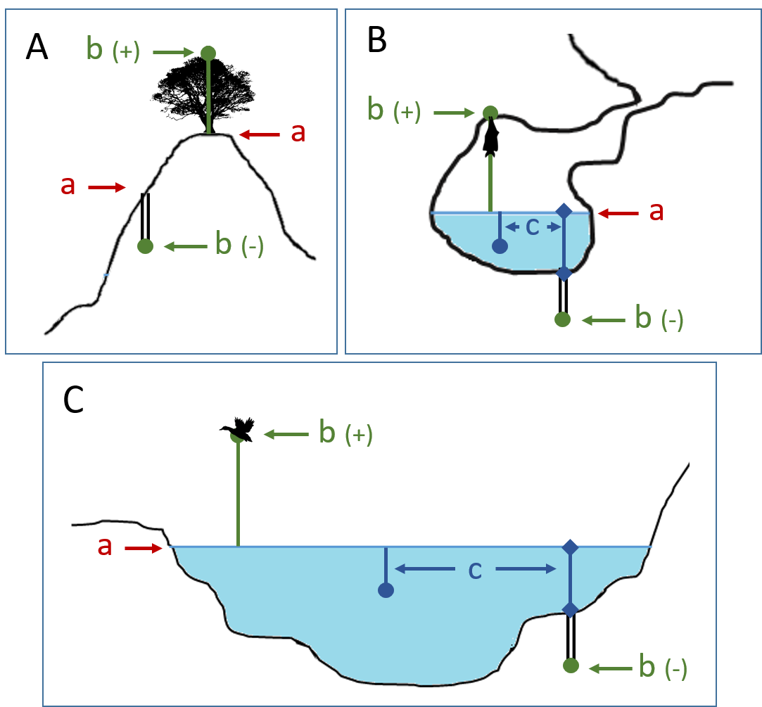
For the special case of recording locations within a cave system or in an underground mine, see §2.12.
2.12. Caves
Collecting in caves, underground mines and tunnels presents a number of challenges not encountered elsewhere.
2.12.1. Determining location
In cave systems and underground mines, determining the geographic position on the surface (known as ground zero) can be done with radiolocation or Electromagnetic Cave-to-Surface (ECMS) Mapping System (Sogade et al. 2004), which uses electromagnetic wave technology. This requires a levelled radio loop in the location within the cave and a receiver above ground to determine the location underground. The surface location can then be determined using a GPS/GNSS receiver, as usual. With a levelled antenna, an experienced operator can determine a ground zero with an accuracy of one meter for a 50 m depth (2%) (Gibson 1996, Gibson 2002), however, more recent radiolocation beacons have increased the horizontal accuracy to about 0.5 to 1 per cent (Goldsheider & Drew 2014, Buecher 2016). Fortunately, many caves and mines have already been extensively mapped, so where maps are available, these may be used to determine locations.
A second method, using the cave mouth, is probably more commonly used, is easier to determine, but is less accurate and has a much greater uncertainty. The cave mouth, tunnel opening, mine shaft entrance, etc., are the most obvious locations to begin with. These locations can easily be obtained using a GPS unit, but be aware of the likely reduced accuracy of the GPS unit if the cave entrance is within a deep valley where good GNSS reception may be reduced. It is documenting the location of the event from that position that is much more difficult, especially where detailed cave maps don’t exist. At its crudest level, one may estimate the cave extent and determine the corrected center of that extent. From there you can determine a geographic radial as noted elsewhere in this document (see §2.3.3). Just recording the location of the cave entrance, and using a large radius for the uncertainty is not ideal but may be a last resort. If doing this however, make sure that your locality description includes as much additional information as possible – such as estimated distance from the cave entrance, direction, and if possible, a ‘depth’. For georeferencing in Caves, see Feature – Cave in Georeferencing Quick Reference Guide (Zermoglio et al. 2020).
2.12.2. Elevation
Traditionally, cavers have recorded the depth in a cave as the depth below the surface, however, in this document and for the purposes of recording biological observations, we use elevation (above mean sea level or geoid) for a position at the floor of the cave.
The distance below ground zero can be determined using the same radiolocation equipment as for determining the ground zero itself (see above). The accuracy of the distance below ground zero, calculated using these methods is around 5-10 per cent (Gibson 1996, Gibson 2002) for depths up to about 50 meters. As above, however, recent beacons have improved the accuracy to about 10 per cent for depths of up to 300 meters below the surface (NOT Engineers 2019). Uneven surface terrain can add to the uncertainties by up to a further 3 per cent and in very deep caves, mines, etc. where there are heavy ore bodies present, and where there are fault lines, this method is far less reliable for determining depth with errors increasing up to 20 per cent. In those conditions radiolocation may not be suitable for determining the distance below the surface.
From these figures, it is possible to determine the elevation of the floor of the cave by taking the elevation at ground zero and deducting the calculated distance below that point (see Figure 10). Note that when determining elevation in a cave, the accuracy mentioned above is additional to the elevation uncertainty determined for the elevation at ground zero.
Using detailed cave maps may provide a better (and cheaper) alternative to other methods, and you should choose the best method for your purpose, but be sure to document how the elevation was determined. Cave maps can usually be obtained by contacting local speleological or cave clubs.
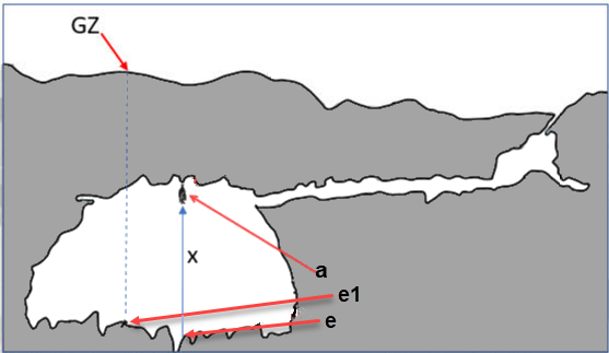
2.12.4. Distance Above or Below a Surface
Determining the distance above (and below) a surface (as documented elsewhere) is treated the same within a cave system (see Figure 9B, Figure 10). As above, the elevation of the cave floor has been determined, so a troglobiont (e.g. an animal) on the roof of the cave is given as meters above the floor of the cave whose elevation has been determined as above ("X" in Figure 10).
2.13. Dealing with Non-natural Occurrences
Records of non-natural occurrences such as cultivated plants and captive animals, and records resulting from beach drift or having been washed ashore (such as shells on a beach that do not contain live animals) should have their "non-natural" or "non-wild" provenance recorded. There may be many valuable uses for these records even if the locations do not correspond to natural occurrences of the organisms. We recommend that the location be recorded and georeferenced, along with the nature of the provenance (cultivated, captive, washed ashore, etc.).
2.14. Absences and Non-Detections
An ‘absence’ is when a particular detection protocol, implemented at a particular location and time, does not result in a detection. True absence occurs in areas where the environmental conditions are unsuitable for a species’ survival. Recording of absences has always been contentious. This is partly because it is very much a result of subjective interpretation and it cannot be vouchered. There are three important and overlapping factors – location, time and methodology. An annual plant, for example, may not be present as an individual at the time of an observation, but may be present at a different time of the year. The location needs to be bounded and is closely linked to the methodology. Uncertainty of the location applies as elsewhere in this document. However, it may have additional implications. Though an observation may record that species x was not detected at a particular location at a particular time using a particular methodology, that location has an uncertainty. The uncertainty is saying that the area within which the observation (non-detection) was made is somewhere within the radius or shape defined by that uncertainty. It does NOT mean that the absence can be ascribed to the totality of the area described by that uncertainty.
There are many methodologies by which an observer may ascribe an absence. Each of these methodologies will have an additional methodological uncertainty associated with it, which is important to record, as it may determine the fitness of that non-detection for a particular use. For example, if you took observations every 10 meters along a transect, and the species was not detected at any of those locations, to what extent can you ascribe an absence to the area covered by the transect? Another methodology may be related to the expertise of the observer. If an expert was intensely searching an area for a species, but at the same time noticed that they hadn’t seen any records of a closely related species, which they would have noticed if it was present – what level of certainty can be given to the surmised observation that the second species is absent from the area?
It is thus important to document:
-
The location as discussed elsewhere in this document
-
The area covered by the non-detection
-
The time, duration, and date
-
The methodology used
2.15. Remotely Captured Data
Counts of animals or plants may be made remotely – for example using an aircraft utilizing direct counts by individuals or using camera or video equipment that is then analyzed back in the laboratory. Examples include aerial counts of kangaroos, counts of whales at sea, etc. It may also include the capture of information from trawls, whereby one or more ships catch marine organisms along one or more paths over a given period (for example, a day) and then the catch is analyzed back on shore. Another example is the use of tracking instruments on birds or turtles, etc. that may give either periodic or intermittent reports of location. Other examples are the use of satellites to remotely image penguins in the Antarctic and then use either individual researchers or machines to count the individual penguins from the satellite image and counts of caribou in the arctic using aerial photography.
In many of these examples, the count of the number of individuals within an area is the aim, rather than the location of individual organisms. This may be recorded as a grid, a polygon, a path, or a line. Record the location, its extent, and the geographic radial for the uncertainty as described for these same geometries in the preceding subsections.
2.16. Data for Small Labels
An issue that often arises with insect collections is the challenge of recording locality information on small labels. This should not be as big an issue as previously, because new technologies allow for linking information on the label to a database (through barcodes, or QR codes, etc.) with the recording of only basic information on the label. See Wheeler et al. 2001 on guidelines for preparing labels for terrestrial arthropods, but bear in mind the principles laid out in this document when preparing data for insect labels, especially the recording of datum, coordinate reference system or EPSG codes, etc., which are not covered by Wheeler et al. 2001.
2.17. Documentation
Record the sources of all measurements. Minimally, include map name and scale, the datum or coordinate reference system, the source for elevation data, the accuracy reported by the GPS receiver, the UTM Zone if using UTM coordinates, the extent and radial of the location, the method used to record the depth, etc.
3. The Georeferencing Process
Locations that are not fully georeferenced in the field may eventually have to be georeferenced after the fact in order to be useful. One hopes in these situations that the collector of the original information followed best practices such as those described in §2. As will be seen in §3.4, below, many of the greatest sources of uncertainty arise from missing, ambiguous, or non-specific information, which could have been avoided, but that can no longer be overcome without knowledge from someone who was there at the time the event occurred.
3.1. Planning a Georeferencing Project
Before beginning a georeferencing project, whether for an individual researcher or a large institution, it is helpful to anticipate the kinds of challenges one might expect to encounter. It may appear to be a daunting task, but there are many ways the process can be simplified and made more practical. Having a suitable workflow (see §3.1.1) decided in advance can increase both the efficiency and the consistency of the quality of the resulting georeferences. The basic determiners for a project are what you have to start with and what outputs you want when you are finished. In an ideal world, the obvious practical questions such as the cost and how long it will take would not be important, but realistically, when balanced against the benefits of making the effort, these might be the major determining factors. Following is a representative list of questions that might affect planning of a georeferencing project:
-
About the original data:
-
Where is the source data coming from (herbarium labels, ledgers, database, or a combination, etc.)
-
Are the source data already digitized?
-
How many distinct locality descriptions are there to georeference?
-
Are there terrestrial or marine locations to georeference? Or both?
-
Is the geographic scope local? Country-wide? Global?
-
-
About the process:
-
What is the time frame for the project?
-
When in the broader workflow will georeferencing happen?
-
How much of the established best practices do I really need to follow?
-
What if we want to use our own methods?
-
What procedural documentation will we need to prepare?
-
Who will do what?
-
What expertise is needed?
-
What skills do those who will be involved possess?
-
Where can training be found?
-
What location resources (maps, gazetteers, tools) are available?
-
-
About the final product:
-
What data quality target is there for the georeferences?
-
How will data validation take place?
-
How will the data be maintained?
-
How will the georeferenced data be used and by whom?
-
Will the georeferences be generalized on export (for sensitive species, for example)?
-
How can the georeferences be integrated back into the original data?
-
How can we incorporate suitable data quality feedback mechanisms?
-
The question, "When in the broader workflow will georeferencing happen?" is of particular significance. Is it best to georeference each record as you enter the data into the database? Or is it better to georeference in a batch after the data have been entered? There are arguments for each method, and again the circumstances of your institution should dictate the best method. If the data are stored taxonomically and not geographically (as is the case in the majority of instances) it is often best to georeference in a batch mode by sorting the locality data electronically, and in this way deal with many records on one map sheet or area at a time and not jump back and forth between map sheets. In other cases, it may be more important to minimize wear and tear on collections, and you may wish to database collections as they are received before distributing duplicates or sending on loan. There may be other good practical reasons to georeference as you go. One advantage of georeferencing as you go is that you may be able to do all the collections of one collector at a time, and virtually follow his/her path, thus reducing errors from not knowing which of several localities may be correct.
This document does not cover methods of general data entry. There are many ways that this may be conducted, including direct entry from the field notes, labels, or ledgers with the material brought to a data entry computer; or direct entry where tablets or laptops are brought to the material. There are also indirect methods, such as entry after using scanning or photographic (still or video) equipment to capture the original information so that data entry can be done after imaging. Capturing the images allows for digitization using handwriting and optical character recognition tools and crowdsourcing (e.g. §4.1, §4.2). Some of these methods are just becoming practical, but you should make an active decision on the method that best suits the needs of your project. When digitization is in progress and each specimen is being handled, it is a good time to consider other actions, such as georeferencing (though we do not recommend this for the sake of efficiency), assigning persistent identifiers (PIDs) (see §1.9), barcoding specimens and linking these to the database to save resources further down the line.
It is also important that the long-term maintenance of the data is considered early in the process. Project managers may wish to consider questions such as:
-
How are we going to deal with corrections to the data?
-
How do we handle feedback on data quality from data aggregators, data users, etc.?
-
Do we have a process in place for documenting changes to the data?
-
Have we budgeted sufficient resources for ongoing maintenance and data quality checking?
3.1.1. Georeferencing Project Workflow
A workflow covering all the georeferencing activities can be a valuable instrument, not only for improving the efficiency of the whole georeferencing process, but also for incorporating checks and balances, and improving the quality of the resulting product. The type of workflow may be determined by the nature of the data, the way the original data are stored or documented, the nature of the desired end product, and even by the general preferences of those involved. In the following subsections we propose a generic workflow that covers all of the major aspects of georeferencing projects. Note that some of the steps presented might not apply to every project, and one must take into account priorities as discussed in §3.1. This first section, §3.1.1 outlines a recommended georeferencing project workflow in four phases. Subsequent sections deal with the details of some of the steps presented in the outline.
Based on an assessment of a variety of large-scale georeferencing projects that had efficiency as well as data quality in mind (e.g. §3.1.2), we recommend the following generic outline for a georeferencing project workflow using either the point-radius method or the shape method, or a mix of the two. This workflow can be used for projects that involve a single individual or a large collaboration, though some steps may apply more in one case than in another. Note that some of the actions included in different phases might happen simultaneously depending on the type and scale of the project.
Project Preparation Phase
-
Commit to the use of a documented set of best practices such as those set forth in this document.
-
Clearly define (and document) the goals of the project, including data quality requirements (see §3.1).
-
Determine what data will be used as input for georeferencing.
-
Select the tools to be used.
-
Estimate the resources needed to complete the georeferencing preparation phase (see §3.1.4).
-
Assign someone to manage the project.
-
Acquire the resources needed to start the project.
Georeferencing Preparation Phase
-
Assemble the data to be georeferenced.
-
Prepare the data for georeferencing:
-
Make sure that original records are uniquely identified (ideally with PIDs, see §1.9).
-
Make sure that original data are captured and safe from alteration during the georeferencing process.
-
Extract distinct combinations of all locality-related fields (including administrative geography, elevation, etc.), generate unique identifiers (ideally GUIDs, see §1.9) for each, and reference the corresponding locality identifier in each original record.
-
Use source-provided administrative geography fields to create and add standardized administrative geography values to the distinct locality records. This will help with the organization of georeferencing by region as well as facilitate lookups against geographic authorities. Optionally, extend this standardization to the contents of the specific locality fields as well. Though this approach has been taken in some large-scale georeferencing efforts such as those undertaken by CONABIO and SiB Colombia (Escobar et al. 2016), there is no clear evidence that the reduction in the number of distinct localities warrants the effort required to do this standardization. More research in this area is needed.
-
Label localities as marine, terrestrial, freshwater aquatic, or paleontological. The same locality description may refer to more than one category (e.g. locations on coasts) unless further constraining information is used (see §3.2.4). If dealing with localities alone, you should account for all of the environmental possibilities.
-
Create and uniquely identify distinct standardized localities and reference the standardized locality GUID in the non-standardized locality records.
-
Match standardized localities against existing localities that have already been georeferenced using satisfactory georeferencing methods and extract the existing georeferences (see §3.1.3).
-
-
Assess the characteristics of the data to be georeferenced (e.g. how many already have coordinates without georeferences? How many consist only of administrative geography? What is the geographic distribution of the localities?) with a view to determining the resources that will be needed to complete the project.
-
Estimate the resources needed to complete the project using the information determined in the project preparation phase.
-
Acquire the resources to complete the project.
-
Train participating contributors and georeferencing operators (see §6.3.1 and §6.6).
-
Establish a convention and tools to manage participation (assignments).
-
Prepare data capture requirements and tools (see §3.1.5, §3.1.7, §3.1.8, and §5.1).
-
Assign priorities to sets of standardized localities.
-
Assign standardized locality sets to participants.
Georeferencing Phase
-
Participants georeference assigned locality sets as outlined in §3.2.
-
Participants utilize protocols and tools such as the Georeferencing Quick Reference Guide (Zermoglio et al. 2020) and the Georeferencing Calculator (Wieczorek & Wieczorek 2020).
Project Follow-up Phase
-
Verify georeferences to meet data quality requirements (e.g. map georeferenced records to ensure they fall in the correct hemisphere, country, etc.) (see §6.3).
-
Populate standardized locality records with data for the georeferences.
-
Normal curatorial activity is not usually suspended during a georeferencing project, which opens the possibility that locality information could be changed for some records in the source database after being aggregated for georeferencing and before being re-incorporated in the source database. For database records that did not have changes to the locality information before re-incorporation, populate the original records from the standardized locality records with georeferences.
-
Repatriate the original records with standardized georeferenced locality data appended to the corresponding institutions (this step is mostly relevant in collaborative projects).
-
Support the incorporation of the standardized georeferenced locality data into the source data management systems (see §6.2).
-
Support the sharing of the standardized georeferenced original data (including additional generalizations and withholdings) in open data venues such as GBIF (see §5).
-
Establish a long-term data maintenance policy that includes the management of feedback on data quality and the documentation of changes (see §6.2).
3.1.2. Project Workflow Example – MaNIS/HerpNET/ORNIS
One of the major contributions of the Mammal Networked Information System (MaNIS) project (Stein & Wieczorek 2004) was the design and implementation of a set of georeferencing guidelines (Wieczorek 2001) and online resources for a collaborative georeferencing workflow. The same basic workflow was implemented with great success for the sister projects HerpNET and the Ornithological Information System (ORNIS). Between the three projects, more than 1.2 million localities were georeferenced for 4.5 million vertebrate occurrence records. The basic workflow was more or less as follows:
-
Establish a georeferencing method and select tools to be used.
-
Train participants (combination of help desk, forum, documents, and in the case of HerpNET, courses).
-
Establish a convention and tools to manage georeferencing work packages for participants.
-
Aggregate occurrences and extract distinct localities into a project gazetteer.
-
Engage participants to claim and complete (georeference) work packages.
-
Participant downloads work package.
-
Participant georeferences work package, consulting documentation and colleagues to resolve questions.
-
Finished work package is sent to the project coordinator.
-
-
Project coordinator validates georeferences to meet data quality standards.
-
Project coordinator populates communal gazetteer with validated georeferences.
-
When georeferencing is completed for the entire project, project coordinator validates that localities for original occurrence records have not changed from the sources since they were added to the gazetteer and repatriates occurrence records with georeferences to participating data custodians.
-
Everyone involved rejoices.
-
Participants add georeference data to their data management systems as time and resources allow.
-
Georeferenced occurrence records get shared via global biodiversity networks such as VertNet (Guralnick & Constable 2010) and GBIF.
3.1.3. Using Previously Georeferenced Records
It may be possible to use a look-up system that searches for similar localities that have already been georeferenced. For example, if you have a record with the locality "10 km NW of Campinas", you can search for all records with locality "Campinas" and see if any records that mean the same thing as "10 km NW of Campinas" have been georeferenced previously. Note that it is always worth verifying the georeference on a map — this can easily be done using software such as Google Maps, Google Earth, etc. Checking this way can reduce errors such as neglecting to add the minus (−) sign to a coordinate in the western or southern hemispheres.
An extension of this method could use the benefits of a distributed data system such as GBIF.org. A search could be conducted to see if the locality has already been georeferenced by another institution. At present, we quite often find that duplicates of occurrence records have been given significantly different georeferences by different institutions. Presumably this would not happen if best practices were followed, or if georeferencing is done by the original institution before distributing duplicates.
A preliminary study (Wieczorek pers. comm.) of roughly 33.1 million occurrences for 38.7 thousand plant taxa in GBIF from 15 April 2019 (GBIF 2019) showed that the records were associated with 7.2 million distinct locations, of which 25.7 per cent (30.9 per cent of occurrences) already had georeferences (i.e. decimalLatitude, decimalLongitude, geodeticDatum and coordinateUncertaintyInMeters). Of those without georeferences, exact matches (on geography plus locality fields, all turned into upper case) from other locations in GBIF could be found for 2.5 per cent of distinct locations (11.4 per cent of occurrences).
In the case where multiple possible georeferences are found using a lookup on previously existing georeferenced locations, the problem is knowing which of the several georeferences, if any, to choose.
If the georeference is not fully documented following best practices (including being reproducible), we recommend that existing georeferences not be used (or used only with extreme caution). Even if the georeference is documented, it should be checked visually on a map to be sure that it makes sense, just as for any new georeference.
| The re-use of existing georeferences can propagate errors, if a mistake was made the first time. Existing georeferences should be verified just as for any newly generated georeference. |
3.1.4. Resources Needed
Each institution will have needs for different resources in order to georeference their location data. The basics, however, include:
-
Suitable computer hardware to support all of the below.
-
A database and database software (spreadsheets may be apt for data capture, but they leave a lot to be desired compared to databases for data management, for which we do not recommend the use of spreadsheets). Note that there are a lot of database management systems already established and available for use with biodiversity data. See if any of these may do the job before developing your own as it may save a lot of extra work. Many also already include data quality aspects that could help improve the quality of your own data.
-
Topographic or bathymetric maps (electronic, paper or both), geologic maps (for paleontological events) and/or speleological maps (for events in cave systems).
-
Access to good gazetteers (many are available free via the Internet, either for downloading, or via online searching).
-
Internet access (as there are many resources on the Internet that will help in georeferencing and locating places).
3.1.5. Data to Capture
One of the most important preparation steps for efficient georeferencing is to have an effective way to handle the data. This section will help you decide if your data capture framework will need modification or not, and to what extent.
Some georeferencing projects (e.g. MaPSTeDI (Murphy et al. 2004)) used a separate working database for data entry operators so that the main data were not modified and day-to-day use of the database was not hindered. This also meant that the working database could be designed optimally for data entry, rather than trying to accommodate other database management and searching requirements. The data from the working database can be checked for quality, and then integrated into the main database from time to time. Such a way of operating is institution dependent, and may be worth considering.
What are the fields you need in your database to best store georeferencing information? This may seem obvious, but it is surprising how often a database is created and finalized before it is determined exactly what the database is supposed to hold. Be sure not to lump together dissimilar data into one field. Always atomize the data into separate fields with very specific definitions and rules for their content.
It is also of benefit to name the fields unambiguously, as users tend to go by the field names rather than looking at the field definitions. Thus, 'latitude_in_degrees' is a better name than 'latitude' for a field that is supposed to contain latitudes in decimal degrees, while 'verbatim_latitude' is better name for a field that is supposed to contain the latitude in the format given in the source. The names and definitions of fields in Darwin Core (Wieczorek et al. 2012b) were created specifically with this principle of clarity in mind. In order to take advantage of a community standard set of definitions, it is not a bad idea to use the term names from Darwin Core as field names in the database if the semantics of the two are the same.
Note, however, that the georeferencing results might benefit from additional fields that are not described in Darwin Core (e.g. 'feature_radial', 'radialUnits') in order to make it easier to reproduce the georeference and thus test its veracity. It is often tempting to include fields for the georeferenced coordinates and ignore any additional fields; however, you (or those who follow after you) are sure to regret this minimalist approach, because it severely limits the usability of the data. A Location occupies a physical extent, not just a point. The associated information on methods used to determine the georeference, the extent, radial, and uncertainty associated with the georeference are important pieces of information for the end user, as well as for managing and improving the quality of your information. The fields that are needed can be divided into two categories: the first consists of the fields associated with the textual description of the location, and the second consists of the fields associated with the spatially enabled interpretation as a georeference and the georeferencing process.
| When atomizing data on entry, always include a field or fields that record the original data in its verbatim form so that atomization and other transformations can later be revealed and checked. |
| Automatic format transformations to decimal degrees may introduce false precision. See §1.6. |
| Be careful with any automatic data formatting or transformation in your database, especially when incorporating original data. Sometimes databases are set to have a particular type or format for data in a given field (e.g. numbers, dates, etc.), which can change the original data and result in irrecoverable losses of information. In this sense, it is recommended that you set all verbatim data fields to be of type "text". Also be aware of the encoding of the data upon import and export, because if the encoding of the data does not match the encoding of the destination, the data can be corrupted. |
| It is always advisable to test the structure of your database with a small sample of records before committing to using it for the whole project. In doing so, you may detect additional fields that are needed and/or fields that require definition review or that are not used at all. |
A reference worth checking before developing your own database system is the Herbarium Information Standards and Protocols for Interchange of Data (Conn 1999, Neish et al. 2007), which, although set up for data interchange between herbaria, is applicable to most data from natural history collections.
Many institutions separate locality descriptions into their component parts; feature name, distance, direction, etc., and store this information in separate fields in their databases. If this division of locality information is done, it is important not to replace the verbatim free-text locality field (the data as written on the label or in the field notebook), but instead add additional fields. This is because any transformation of data has the potential to lose information and to introduce errors, and the written format of the description may be the only original source available. The original information should never be overwritten or deleted.
Location-related fields to consider for georeferencing include all of the geography, locality, elevation, depth, and georeference terms in the Location class of Darwin Core (see location and §5.1) as well as the following fields that can have an influence on the georeference:
-
As many levels of administrative subdivision as necessary (e.g. country, state, county, municipality, etc.), though if the geographic scope is multinational, it is better to name the administrative subdivisions more generically to avoid confusion (e.g. country, geog_admin_1, geog_admin_2, etc.)
-
Feature name, feature-type, offset distance, offset direction, offset units
-
Feature shape, feature center, feature radial
-
Township, range, section, subsection or similar for other grid systems
-
Protected area
-
Watershed
-
Map quad
-
Universal Transverse Mercator (UTM) easting, northing, and zone
-
For
marine locations - nearest island, exclusive economic zone, etc. -
Elevation accuracy, vertical datum, and the method of determining elevation
-
Depth accuracy, vertical datum, and the method of determining depth
-
Latitude degrees, latitude minutes, latitude seconds, latitude hemisphere, longitude degrees, longitude minutes, longitude seconds, longitude hemisphere
-
Biome, to distinguish terrestrial, freshwater aquatic, and marine locations
-
Event date (best to follow and enforce a standard format, such as ISO 8601 (ISO 2019). Note that if your project is dealing with location information only (dissociated from occurrence or event records), this may not be possible or advisable.
-
Fields in the Darwin Core GeologicalContext class for paleontological occurrences
| When adding extra fields to your database, always consider that the more fields you add, the higher the chances that data entry operators could make a mistake. Therefore, although having more fields has many advantages when it comes to checking the results, try to avoid over parsing information if not really necessary. |
3.1.6. Applying Data Constraints
One of the key ways of making sure that data are standardized and accurate is to ensure, to the extent possible, that data are put in the correct field and that only data of an appropriate type can be put into each field by design. This is done by applying constraints on the data fields – for example, only allowing values between +90 and −90 in the field for decimal latitude. Many of the errors found when checking databases could have been easily avoided if the database had been set up correctly in the first place. The use of pick lists is essential where the field should contain only values from a restricted list of terms.
More complex constraints may also be possible. With ecological or survey data for example, one could set boundary limits between the starting locality and ending locality of a transect. For example, if your methodology always uses 1 km or shorter transects, then the database could include a boundary limit that flagged whenever an attempt was made to place these two points more than 1 km apart.
For more information on constraints, see various sections under §3.4.1.
3.1.7. User Interfaces
Good user-friendly interfaces are essential to make georeferencing efficient and rapid, and to cut down on operator errors. The design should take into consideration the specific details of the georeferencing workflow, and optimize simultaneously for both overall efficiency, and consistency of the data entry process. This will improve accuracy and cut down on errors. The layout should be friendly, easy to use, and easy on the eyes. Where possible (and the software allows it) a number of different views of the data should be presented. These views can place emphasis on different aspects of the data and help data entry operator proficiency by allowing different ways of entering the data and by presenting a changing view for the operator.
In the same way, macros and scripts can help with automated and semi-automated procedures, reducing the need for tedious (and time-consuming) repetition. For example, if the data are being entered from a number of collections by one collector, taken at the same time from the same location, the information that is repeated from record to record should be able to be entered using just one or two keystrokes.
If maps are being used to assist in determining georeferences, a view that sorts the data geographically may also make the process more efficient by allowing the data operator to see all the records that may fall on one map sheet. Finally, it is also important to decide which fields the data entry operators should see when they are georeferencing. Fields such as date of collection, collector, specimen ID, taxonomy, habitat, and formation (for paleontological records) are very helpful for georeferencers to see along with the more obvious locality data.
3.1.8. Using Standards and Guidelines
Standard methodologies, in-house standards, and guidelines can help lead to consistency throughout the database and cut down on errors. A set of standards and guidelines should be established before any georeferencing begins (see §2.17). They should remain flexible enough to cater for new data and changes in processes over time, though careful thought beforehand can minimize the need for methodological changes, which might lead to inconsistencies where earlier efforts are lacking compared to those produced under newer protocols. Standards and guidelines in the following areas can improve the quality of the data and the efficiency of data entry:
-
Units of measure. Use a single unit of measure in interpreted fields. For example, do not allow a mixture of feet and meters in elevation and depth fields. Irrespective of this, the original units and measurements should be retained in a verbatim field.
-
Methods and formats for determining and recording uncertainty and extent.
-
Required fields (fields that must have meaningful, non-empty values).
-
Format for recording coordinates (e.g. degrees/minutes/seconds, degrees/decimal minutes, or decimal degrees for latitude and longitude).
-
Original source(s) of place names and features.
-
Dealing with typographical errors and other errors in the existing database.
-
Number of decimal places to keep in the various fields with decimal numbers.
-
How to deal with "empty" values as opposed to the numerical value zero (Note: configure databases to not supply 0 for an empty value).
-
How to deal with mandatory fields that cannot be filled in immediately (e.g. because a reference has to be found). There may be a need for a default value that flags that the information is still required.
-
Methods for data validation that will be carried out before a record can be considered complete and verified.
Determining and documenting your institution’s own georeferencing best practice in manuals, for example that suit the circumstances of that institute (including language, local software and resources, etc.) can help maintain consistency as well as assist in training and data quality recording. As an example, see Escobar et al. 2015, where an internal document for the Alexander von Humboldt Institute in Colombia has been developed and put into practice. See also §2.17.
3.1.9. Data Entry Operators
One of the greatest sources of georeferencing error is the data entry process. It is important that this process is made user-friendly and set up so that many errors cannot occur (e.g. through the use of pick lists, field constraints, etc.). The selection and training of data entry operators (see under §6.6) can make a big difference to the final quality of the georeferenced data. As mentioned earlier, the provision of good guidelines and standards can help in the training process and allow for data entry operators to reinforce their training over time.
3.2. Georeferencing Workflow – Localities
At the heart of any georeferencing project is the hands-on georeferencing of individual locality descriptions. The value of getting this part right can’t be overstated.
Regardless of what other steps might have preceded this in a project workflow, for individual localities we recommend the following georeferencing workflow — refined from Wieczorek et al. 2004.
-
Choose the georeferencing method (e.g. point-radius, bounding box, shape) to use. You may do this for all localities or on a case by case basis (see §3.3).
-
Parse the locality into locality clauses (see §3.2.1).
-
Identify the feature(s) and determine the locality type of the most specific locality clause (see §3.2.2).
-
Find the feature(s) in a spatial data source (e.g. map, gazetteer, GIS layer, application programming interface (API)) that can give you an idea of where the feature is with coordinates, a bounding box, a point-radius, or a shape).
-
Determine the boundaries of the feature(s) (see §3.2.3) including all constraints (see §3.2.4).
-
Follow the protocol in the Georeferencing Quick Reference Guide (Zermoglio et al. 2020) to georeference the locality based on the locality type of the most specific clause and the shape or point-radius of the constrained feature from the previous step.
-
Document the sources and methods sufficiently to make the resulting georeference reproducible (see §1.1).
Though the list of steps above applies to a single locality record, the most efficient way to implement these steps might be to do each step for all of the localities in the set, and use the results of that step to organize the next step. For example, by identifying the features from all of the most specific clauses, one could filter localities by feature and with the accumulated body of information about the feature from all the localities at hand, georeference all of the localities containing the same feature together. One could also do statistics on the number of records affected by determining the boundaries of each feature and use that to prioritize which localities get georeferenced, if resources do not otherwise cover georeferencing everything. This kind of feature extraction could be done in the aggregate georeferencing preparation stage (see §3.1.1).
3.2.1. Parsing the Locality Description
Locality descriptions are often given in free text and encompass a wide range of content in a vast array of formats. An important part of the georeferencing process is to have a consistent way to interpret the text into spatial forms that can be operated on analytically. To do this, look for the parts of the description that can be interpreted independently, called locality clauses, each of which can be categorized into a locality type (see §3.2.2) that uses a specific set of rules to georeference (Wieczorek et al. 2004).
3.2.2. Classifying the Locality Description
There is a lot of variation in the way clauses are written and the types of features they reference, but there are actually very few basic locality types, though these may have many variations depending on the feature type referenced. The Georeferencing Quick Reference Guide (Zermoglio et al. 2020) was written specifically to explain how to georeference all of the most common variations of locality types and feature types (Wieczorek et al. 2004):
-
coordinates only (e.g. 27°34'23.4" N, 121°56'42.3" W)
-
geographic feature only (e.g. "Bakersfield")
-
distance only (e.g. "5 mi from Bakersfield")
-
heading only (e.g. "North of Bakersfield")
-
distance along a path (e.g. "13 miles east (by road) from Bakersfield")
-
distance along orthogonal directions (e.g. "2 miles east and 3 miles north of Bakersfield")
-
distance at a heading (e.g. "10 miles east (by air) from Bakersfield")
-
distances from two distinct paths (e.g. "1.5 miles east of Louisiana State Highway 1026 and 2 miles south of U.S. Highway 190")
-
dubious (e.g. "presumably central Chile")
-
cannot be located (e.g. "locality not recorded")
-
demonstrably inconsistent (e.g. "Sonoma County side of the Gualala River, Mendocino County")
-
captive or cultivated (e.g. "San Diego Wild Animal Park")
A full locality description may contain multiple clauses. The goal of a georeference is to describe the location where all of the clauses are true simultaneously. In GIS terms, this would be the intersection of the shapes for all the clauses in the locality description. As humans, we would choose the clause that is most specific and georeference based on that, using the information from the other clauses to filter from among multiple possibilities. For example, a locality written as
bridge over the St. Croix River, 4 km N of Somerset
should be georeferenced with a locality type "geographic feature only" with subtype Feature – with Obvious Spatial Extent as in Georeferencing Quick Reference Guide (Zermoglio et al. 2020) based on the bridge as the feature. Of course, the second clause helps us to determine which bridge (something we wouldn’t be able to do without that second clause), but beyond that the second clause contributes nothing to the boundaries of the feature, nor to the uncertainty in the final georeference.
If the more specific part of the locality cannot be unambiguously identified, then the next less specific part of the locality ("4 km N of Somerset" in the example above) should be georeferenced. In a case such as this, annotate in the georeference remarks with something like "unable to find the bridge georeferenced '4 km N of Somerset'".
Some locality descriptions give information about the nature of the offset (‘by road’, ‘by river’, ‘by air’, ‘up the valley’, etc.). Having this information simplifies the choice of offset-based locality type as §2.9.3 or §2.9.4.
|
|
|
|
|
|
|
|
In this example, there are four fields contributing five separate clauses. The three administrative geography terms each have one clause of the type "Geographic feature only" with subtype "Feature – with obvious spatial extent" (see Feature – with Obvious Spatial Extent in Georeferencing Quick Reference Guide (Zermoglio et al. 2020)), while the locality field contains a clause ("12.3 km N of (by road) Nahuel Huapi") of the type "Distance along path" (see Offset – Distance along a Path in Georeferencing Quick Reference Guide) and a clause ("elev: 760m") of the type "Geographic feature only" with subtype "Feature – Path" (see Feature – Path in Georeferencing Quick Reference Guide). The most specific of all five clauses is "12.3 km N of (by road) Nahuel Huapi".
It is sometimes possible to infer the nature of the offset path from additional supporting evidence in the locality description. For example, the locality
58 km NW of Haines Junction, Kluane Lake
suggests a measurement by road since the final coordinates by that path are nearer to the lake than going 58 km NW in a straight line. At other times, you may have to consult detailed supplementary sources, such as field notes, collectors’ itineraries (see §3.2.4.4), diaries, or sequential collections made on the same day, to determine this information.
If any of the clauses in the locality description is classified as one of the three locality types, ‘dubious’, ‘cannot be located’, or ‘demonstrably inaccurate’, then the locality should not be georeferenced. Instead, an annotation should be made to the locality record giving the reason why it is not being georeferenced. See also Difficult Localities in Georeferencing Quick Reference Guide (Zermoglio et al. 2020).
3.2.3. Setting the Boundaries of the Feature
Regardless of the method to be used (shape, bounding box, or point-radius), the georeferencing protocols for nearly every locality type begin with the identification of the features of reference in the locality description and the determination of the geographic boundaries of their extents. This is usually the most critical and time-consuming part of the protocols. It is best to use a visual reference to determine boundaries. If a feature name search on a visual source does not reveal the feature of interest, it is a good idea to use coordinates from a gazetteer to find the feature on a map, and then use the map to find the boundaries:
-
Point-radius method: store the corrected center of the constrained boundaries from the previous step as decimal latitude and decimal longitude and store the geographic radial as a distance in the units given in the most specific locality clause. If there are no distance units in that clause, use meters (see §3.3.2).
-
Bounding Box method: store the furthest north, south, east, and west coordinates on the constrained boundaries of the feature (see §3.3.3).
-
Shape method: store the resulting constrained boundaries as a shape (see §3.3.4).
3.2.4. Applying Spatial Constraints
There are many ways that a location can be constrained beyond what the geography and locality descriptions alone suggest. Doing so relies on applying additional location information, such as elevation or depth, lithostratigraphic information for fossils, or information outside the location information, such as environmental constraints for a particular species. There are important implications about workflow and effort that need to be considered when applying additional constraints. For example, if taxon constraints are going to be applied, the georeferencing cannot be done strictly on location information, which means it has to be done on occurrence records, or on an index combining location and taxon. This would be much slower than georeferencing based on location alone. A good compromise would be to georeference in multiple stages, with the first stage based on location information, and a subsequent stage including the rest of the occurrence information, and perhaps a final stage of review by collectors to be able to set dwc:georeferenceVerificationStatus to "verified by collector" – the best status a georeference can possibly have.
Taxon Constraints
It is common to encounter locality descriptions for which the boundaries and uncertainty could be reduced if the taxon and its environmental or geographic constraints are known.
One case in which a taxon constraint might be applied is where a locality description would be georeferenced in a distinct manner if it was known to be terrestrial, aquatic, or marine. Here even the life stage of a taxon could be taken into account.
OBIS (the Ocean Biodiversity Information System) uses the World Register of Marine Species (WoRMS 2019) to determine if a species can be classified as either marine or terrestrial. Note, however, that there are many species listed in the WoRMS database that occur on coastal shores or in estuaries (i.e. species that could be regarded as both marine and terrestrial at some stage during their life cycle), so caution needs to be taken when using this method in georeferencing.
At the generic level there are similar biome-matching services available through the Interim Register of Marine and Nonmarine Genera (IRMNG) (Rees 2019), and the associated LifeWatch taxon matching services.
Another case where taxon might be taken into account is where a distribution range or environmental domain suggests a restriction in the boundaries of a location. However, this kind of constraint on a georeference is not recommended, because an organism whose location falls outside of an established range map may indicate a genuine outlier, or a taxon misidentification. Given that, such information can help distinguish between two possible locations of the same feature name where one possible location fits within the environmental domain for the taxon, and the other outside the range. This auxiliary information is also particularly useful after georeferencing, to reveal records of possible range extensions, exotic invasions, or cryptic taxa.
Using Date Constraints
The date is an important characteristic of an event and must be recorded. Towns, roads, counties, and even countries can change names and boundaries over time, and can even cease to exist as extant features. Rivers and coastlines can change position, billabongs and ox-bow lakes can come and go, and areas of once pristine environment may become farmland or urban areas.
“Collecting localities along the Alaska Highway are frequently given in terms of milepost markers; however, the Alaska Highway is approximately 40 km shorter than it was in 1942 and road improvements continue to re-route and shorten it every year. Accurate location of a milepost, therefore, would require cross-referencing to the collecting date. To further complicate matters, Alaska uses historical mileposts (calibrated to 1942 distance), the Yukon uses historical mileposts converted to kilometers, and British Columbia uses actual mileage (expressed in kilometers).” From Wheeler et al. 2001
To the extent possible, the aim is to have a georeference and its uncertainties based on the conditions at the time an event occurred at a locality. There are two major implications associated with this. One is that current maps and gazetteers may not reflect the conditions at the time of the event, and the other is that old maps and gazetteers may not represent well the conditions of later events.
We recommend that this sort of constraint be used in a followup workflow step to deal with localities at the event level rather than try to construct a gazetteer that includes collecting dates.
Using Elevation or Depth Constraints
Elevation can often be used as a constraint to distinguish between two similarly named localities or to refine the uncertainty in a georeference. If both maximum and minimum elevations are given, then the contours of these limits may be used to constrain the extent of a locality and therefore its uncertainty. If a single value is given for elevation, then the precision of that value can be used to estimate the minimum and maximum elevations as described in §3.4.6 Uncertainty Related to Offset Precision. The Georeferencing Quick Reference Guide (Zermoglio et al. 2020) describes how to georeference using elevation constraints in section 2.1.3.3. Feature – Path. The same considerations can also be applied to occurrence depths in cases of benthic organisms, or when the depth of the waterbody floor is available in non-benthic occurrence records, or to exclude geographic regions where waterbody depth is shallower than occurrence depth given.
Using Collector Itineraries
Collector’s itineraries and expedition tracks can be a useful adjunct in discovering locations that are otherwise difficult to find, especially where there may be more than one possible location based on a feature name. This may be done through using field notebooks, published reports and maps, searching for the localities of specimens with adjacent collecting numbers, etc. With historic collecting events (i.e. before the days of modern transport), you may also be able to restrict the area to look in by limiting the distance a collector may have been able to travel within one day. Note that the collector name and date are essential pieces of information in tracking itineraries, and therefore can not be done on localities alone. We thus recommend that this sort of constraint be used in a followup workflow step to deal with unresolved localities rather than try to construct a gazetteer that includes collecting dates, collector names, and collector numbers.
Using Ship Logs
Digitized ships logs contain a wealth of data (Dempsey 2014) and are valuable data resources. A freely downloadable database of surface marine observational records from ships, buoys, and other platform types is available as the International Comprehensive Ocean-Atmosphere Data Set (NOAA 2018). Be aware that the accuracy of records obtained from this dataset vary, depending on the original source, and are not always documented.
Using Geological Context
Maps or GIS layers of geological contexts, such as formations, can be used to narrow the location in the case of a paleontological specimen that includes such information in the shared content of the record. For example, if a fossil is taken from the surface in the Fox Hills formation (which is Cretaceous in age), that can distinguish the location from nearby different formations on the surface, like a habitat could do in an ecological context.
3.3. Georeferencing Methods
The distinction between georeferencing methods is in the basic approach taken to capture spatially enabled location data. Within each method there should be protocols for how to produce georeferences based on the input locality description and supporting information. The goal of any georeferencing method and its specific, documented protocols should be to create a spatial representation of the entire location, including all uncertainties involved, with sufficient accompanying information and documentation to make the georeference reproducible.
3.3.1. Point Method
Based on the aspirations for georeferencing methods described in the previous paragraph, the point method, consisting of only coordinates, or coordinates in a coordinate reference system, is insufficient to be useful except to center a point on a map (and even that potentially incorrectly without the coordinate reference system). The point method does not give any indication of scale, though the mistake is often made to try to represent scale and/or uncertainties in the precision of the coordinates. For these reasons, the point method is NOT recommended as the end product of a georeferencing workflow.
3.3.2. Point-radius Method
The result of the point-radius method (Wieczorek et al. 2004) is a geographic coordinate (the "corrected center"), its geodetic datum, and a maximum uncertainty distance as a radius. The length of the radius must be large enough so that a circle centered on the corrected center and based on that radius encompasses all of the uncertainties in the interpretation of the location. The point-radius is a very simple representation of the location that contains all of the places that the locality description might refer to, but may also circumscribe areas that do not match the locality description. That’s OK. The point-radius circle can also be intersected with other spatially enabled information to constrain the effective area within the circle, such as elevation, to derive a shape representation of the locality. For example, calculate the intersection of a point-radius circle with the shape of the matching elevation contours in a geographic information system to get a shape that better matches the described locality. Similarly, one could calculate the intersection of an exposed geological formation with a point-radius georeference to refine the latter into a shape. The detailed recommended protocols for georeferencing using the point-radius method are given in the Georeferencing Quick Reference Guide (Zermoglio et al. 2020).
3.3.3. Bounding Box Method
The result of the bounding box method (Wieczorek et al. 2004) is a set of two coordinates, one for each of two corners diagonally opposed on the bounding box along with their coordinate reference system. The corners define the minimum and maximum values of the coordinates, within which the whole of the location and its uncertainties is contained. Like the point-radius method, the bounding box method results in a very simple representation of the location that contains all of the places that the locality description might refer to, but may also contain areas that do not match the locality description.
Unlike the point-radius method, this method has no scalar maximum uncertainty distance to be able to easily understand or filter on the size of the enclosed region, though one can be calculated using half the distance between the two corners as given by Vincenty’s formulae (Vincenty 1975, Vincenty 1976). Thus, a bounding box georeference can be turned into a point-radius georeference by using the distance just described as the geographic radial, and from that finding the corrected center, which will not be equal to the geographic center of the bounding box, except where the bounding box spans equal distances north and south of the equator or is based on a metric grid.
A point-radius georeference can be turned into a bounding box georeference by using the geographic radial from the corrected center of the point-radius to determine the coordinates of the east-west and north-south extremes of the bounding box.
| Though transformations can be made back and forth between point-radius and bounding box representations of a location, it is not recommended, because the transformed georeference will necessarily be bigger than the original, and therefore contain more area that does not pertain to the actual location. Better to georeference directly using the method of choice. |
Like the point-radius circle, the bounding box can also be intersected with other spatially enabled information to constrain the effective area within.
3.3.4. Shape Method
The shape method (also called the polygon method by some (Yost 2015)) of determining uncertainty is a conceptually simple method that delineates a locality using geometries with one or more polygons, buffered points, or buffered polylines. A combination of these shapes can represent a town, park, river, junction, or any other feature or combination of features found on a map. While simple to describe, the task of generating these shapes must account for all the uncertainties, and that can be difficult. Except for the simplest locality types, creating shapes is impractical without the aid of digital maps, GIS software (for buffering, clipping, etc.), and expertise, all of which can be relatively expensive. Also, except for a bounding box, which is an extremely simple example, storing a shape in a database can be considerably more complicated than storing a single pair of coordinates with a scalar uncertainty distance as in the point-radius method. Darwin Core (Wieczorek et al. 2012b) offers the field dwc:footprintWKT, in which a geometry can be stored in the Well-Known Text format (ISO 2016) accompanied by the coordinate reference system in the field dwc:footprintSRS. Particular challenges to making this method practical for georeferencing natural history collections data include assembling freely accessible digital cartographic resources and developing tools for automation of the georeferencing process (Yost n.d.). This is because, not only does the geometry of the feature usually need to be created (unless it is an administrative boundary or other shape available in a spatial data layer), but also all the points in the feature geometry have to be used in combination with the uncertainties to arrive at a final shape that includes the location with its uncertainties and nothing more. Note that GEOLocate (Rios 2019) does produce an "error polygon" (Biedron & Famoso 2016) in addition to a point-radius, but how this is done is not documented in detail.
Of all the methods discussed in this document, the shape method has the potential to generate the most specific digital spatial descriptions of localities, leaving out areas that are not viable as part of the location. A point-radius can be easily derived from a final shape by using the corrected center for the coordinates and the geographic radial of the georeference (not just the feature) for the maximum uncertainty distance. See Figure 15 for one example of where a point-radius may be refined by using the shape method. See also §2.3.3.
3.3.5. Probabilistic Method
Other shape-based methods have been proposed that use probabilistic approaches (Guo et al. 2008, Liu et al. 2009). Since these methods are even more difficult than the shape method, and there are currently no tools available to take advantage of these methods, we do not discuss them further in this document.
3.4. Calculating Uncertainties
Regardless of the method, uncertainties in georeferenced data are essential to document, so that the data’s fitness for use and thus their overall data quality can be understood. There are sources of uncertainty in each locality interpretation as well as in the data sources used to georeference, and any physical measurement that might need to be made (such as on maps, digital or physical). Each of the sources of uncertainty have to be taken into account to capture the overall uncertainty in a resulting georeference.
Whenever subjectivity is involved, it is preferable to overestimate each contribution to uncertainty. The following seven sources of uncertainty are the most commonly encountered. These are explained below and can be accounted for by using the Georeferencing Calculator (Wieczorek & Wieczorek 2020).
-
Uncertainty due to the extent of the feature in the locality description.
-
Uncertainty in coordinate source.
-
Uncertainty in map measurements.
-
Uncertainty related to coordinate precision.
-
Uncertainty from unknown coordinate reference system or datum.
-
Uncertainty related to heading.
3.4.1. Uncertainty Due to the Extent of the Feature
The first step in determining the coordinates for a locality description is to identify the most specific feature within the locality description. Coordinates may be retrieved from gazetteers, geographic name databases, maps, or from other locality descriptions that have coordinates or shapes. We use the term ‘feature’ to refer to not only traditional named places, but also to places that may not have proper names, such as road junctions, stream confluences, highway mile pegs, and cells in grid systems (e.g. Quarter Degree Square Cells, see §2.3.4.2). The source and precision of the coordinates should be recorded so that the validity of the georeferenced locality can be checked. The original coordinate system and the geodetic datum should also be recorded. This information helps to determine sources and the maximum uncertainty distance, especially with respect to the original coordinate precision.
How do we take into account the uncertainty due to the shape of the feature? The method that results in the least uncertainty is to find the smallest enclosing circle (Matoušek et al. 1996) that contains all of the points on the geographic boundary of the feature. If the center of the circle does not fall on or within the boundary of the feature, choose the point nearest to the center that is on the boundary. This is known as the corrected center. The distance from the corrected center to the farthest point on the geographic boundary of the feature is called the geographic radial. The geographic radial is the uncertainty due to the extent of the feature (see Figure 4).
Every feature occupies a finite space, or ‘extent’. The extents of features are an important source of uncertainty. Points of reference for features may change over time – post offices and courthouses are relocated, towns change in size, the courses of rivers change, etc. Moreover, there is no guarantee that the person who recorded the locality information paid attention to any specific convention when reporting a locality as an offset from a feature. For example,
4 km E of Bariloche, Argentina
may have been measured from the post office, the civic plaza, or from the bus station on the eastern side of the heavily populated part of town, or anywhere else in Bariloche, which is actually quite large. When calculating an offset, we generally have no way of knowing where the person who recorded the locality started to measure the distance. The determination of the boundaries of a feature are discussed in §3.2.3.
It is also worth noting that the extent of a feature may have changed over time, so the date of the recording may also be important when calculating an extent and thus the geographic radial. In many cases (especially for populated places), the current extent of a feature will be greater than its historical extent and the uncertainty may be somewhat overestimated if current maps are used.
If the locality described is an irregular shape (e.g. a winding road or river), there are two ways of calculating the "center" coordinates and determining the radial. The first is to measure along the vector (line) and determine the midpoint as the location of the feature. This is not always easy, so the second method is to determine the geographic center (i.e. the midpoint of the extremes of latitude and longitude) of the feature. This method describes a point where the uncertainty due to the extent of the feature is minimized (what we are calling the corrected center). The radial is then determined as the distance from the determined position to the furthest point at the extremes of the vector. If the geographic center of the shape is used and it does not lie within the locality described (e.g. the geographic center of a segment of a river does not actually lie on the river), then the point nearest the geographic center that lies within the shape (corrected center) is the preferred reference for the feature and represents the point from which the geographic radial should be calculated (see Figure 4).
When documenting the georeferencing process, it is recommended that the feature, its extent, radial, and the source of the information (including its date) all be recorded. For details on georeferencing, see Geographic Feature Only in Georeferencing Quick Reference Guide (Zermoglio et al. 2020).
Geographic coordinates can be expressed in a number of different coordinate formats. Decimal degrees provide the most convenient coordinates to use for georeferencing for no more profound reason than a locality can be described with only four attributes – decimal latitude, decimal longitude, datum, and uncertainty (Wieczorek 2001).
3.4.2. Uncertainty in Coordinate Source
There are many ways of finding coordinates for a location, including using a gazetteer, a GPS, aerial photogrammetry, digital maps, or paper maps of many different types, and scales.
Uncertainty in Paper Map Measurements
One of the most common methods of finding coordinates for a location is to estimate the location from a paper map. Using paper maps can be problematic and subject to varying degrees of inaccuracy. Unfortunately, the accuracy of many maps, particularly old ones, is undocumented. Accuracy standards generally explain the physical error tolerance on a printed map, so that the net uncertainty is dependent on the map scale (see Table 1).
Map reading requires a certain level of skill in order to determine coordinates accurately, and different types of maps require different skills. Challenges arise due to the coordinate system of the map (latitude and longitude, Universal Transverse Mercator (UTM), etc.), the scale of the paper map, the line widths used to draw the features on the maps, the frequency of grid lines, etc.
The accuracy of a map depends on the accuracy of the original data used to compile the map, how accurately these source data have been transferred onto the map, and the resolution at which the map is printed or displayed. For example, USGS maps of 1:24,000 and 1:100,000 are different products. The accuracy is explicitly dependent on scale but is due to the different methods of preparation. When using a map, the user must take into account the limitations encountered by the map maker such as acuity of vision, lithographic processes, plotting methodologies, and symbolization of features (e.g. line widths) (Hardy & Field 2012).
With paper topographic maps, drawing constraints may restrict the accuracy with which lines are placed on the map. A 0.5 mm wide line depicting a road on a 1:250,000 map represents 125 meters on the ground. To depict a railway running beside the road, a separation of 1-2 mm (250-500 meters) is needed, and then the line for the railway (another 0.5 mm or 125 meters) makes a total of 500-750 m as a minimum representation. If one uses such features to determine an occurrence locality, for example, then minimum uncertainty would be in the order of 1 km. If thicker lines were used, then appropriate adjustments would need to be made (Chapman et al. 2005).
The National Standard for Spatial Data Accuracy (NSSDA) (FGDC 1998) established a standard methodology for calculating the horizontal and vertical accuracy of printed maps, which state that 95% of all points must fall within a specified tolerance (1/30" for map scales larger than 1:20,000, and 1/50" for map scales smaller than or equal to 1:20,000).
Table 1 shows the inherent accuracy of a number of maps at different scales. The table gives uncertainties for a line 0.5 mm wide at a number of different map scales. A value of 1 mm of error can be used on maps for which the standards are not published. This corresponds to about three times the detectable graphical error and should serve well as an uncertainty estimate for most maps.
The table uses data from several sources. The TOPO250K Map series is the finest resolution mapping that covers the whole of the Australian continent. It is based on 1:250,000 topographic data, for which Geoscience Australia 2007, Section 2 defines the accuracy as "not more than 10% of well-defined features are in error by more than 140 meters (for 1:250,000 scale maps); more than 56 meters (for 1:100,000 maps)". The USGS Map Horizontal Uncertainty is calculated from US Bureau of Budget (1947) (reported in United States National Map Accuracy Standards (USGS 1999)) which states that "As applied to the USGS 7.5-minute quadrangle topographic map, the horizontal accuracy standard requires that the positions of 90 percent of all points tested must be accurate within 1/50th of an inch (0.05 centimeters) on the map. At 1:24,000 scale, 1/50th of an inch is 40 feet (12.2 meters)." These values need to be taken into account when determining the uncertainty of your georeference.
| Scale of Map | Map Horizontal Accuracy (Geoscience Australia) | Map Horizontal Accuracy (USGS) | NSSDA Horizontal Accuracy (FGDC 1998) |
|---|---|---|---|
1:1000 |
0.5 m |
2.8 ft (0.85 m) |
3.2 ft (1 m) |
1:10,000 |
5 m |
28 ft (8.5 m) |
32 ft (10 m) |
1:25,000 |
12.5 m |
70 ft (21 m) |
47.5 ft (14.5 m) |
1:50,000 |
25 m |
139 ft (42 m) |
95 ft (29 m) |
1:75,000 |
142.5 ft (43.5 m) |
||
1:100,000 |
50 m |
278 ft (85 m) |
190 ft (58 m) |
1:250,000 |
160-300 m |
695 ft (210 m) |
475 ft (145 m) |
1:500,000 |
950 ft (290 m) |
||
1:1 million |
500 m |
2,777 ft (845 m) |
1,900 ft (580 m) |
If you are using phenomena that do not have distinct boundaries in nature to determine a locality (such as soils, vegetation, geology, timberlines, etc.) then err vastly on the side of conservatism when determining an uncertainty value as such boundaries are seldom accurate, often determined at a scale of 1:1 million or worse and would have a minimum uncertainty of between 1 and 5 km. Also be aware that coastlines vary greatly at different scales (see Chapman et al. 2005) and rivers are often straightened on smaller scale maps, and can thus include uncertainties far greater than are generally recorded on maps whose accuracies are determined from "well-defined" points such as buildings, road intersections, etc. In addition, coastlines and river paths can change greatly over time (World Ocean Review 2010) and thus the date of the map needs to be taken into account when determining uncertainty.
In addition to the inherent inaccuracies of printed maps, one must consider inaccuracies that can arise from using maps to measure distances. These potential inaccuracies are a direct consequence of the projection of the map and one’s ability to distinguish between two adjacent points, which may be affected by your measuring device and even your eyesight. A straight line distance measurement only works on a map in an equal distance projection, where distance follows the same scale regardless of the orientation. Unless the conditions for measuring are particularly poor, it is reasonable to use 1 mm as a value for measurement error on physical maps. Depending on the scale of the map, this translates into a distance on the ground.
Uncertainty in Digital Map Measurements
Digital versions of traditional paper maps that have been scanned or digitized by hand using a digitizing tablet to trace lines, have an extra layer of uncertainty (Dempsey 2017). Depending on how the map was digitized, the error may be small or large when compared to the scale of the original map. In parts of the world where digitized maps are not readily available, they can be scanned and rectified using satellite data (Raes et al. 2009). Scanned maps often (and should always) include information on the accuracy added by the digitizing process (see ASPRS 1990). Be careful when using digital maps, and record any information on the scanning accuracy if that information is available. Always err on the cautious side when recording the uncertainty of your georeference when using maps of this type (ASPRS 2014).
| A digital map is never more accurate than the original from which it was derived, nor is it more accurate when you zoom in on it. The accuracy is strictly a function of the scale and digitizing errors of the original map, plus the additional error added by the digitization process. |
| Care must be used when using a digital map that records the scale in the form of text (e.g. 1:100,000) rather than by using a scale bar, as the resolution of the computer screen, and the level of zooming will change the apparent scale of the map being viewed. (It does not change the scale at which the map was prepared). This also applies to maps printed from a digital map. When preparing digital maps, always include scale as a scale bar and do not just record scale in textual form (e.g. 1:20,000). |
Measurement error is not unique to physical maps, it also enters into measurements on digital media. In general, the resolution of the media affects one’s ability to distinguish between two points, and this in turn can be affected by the extent to which the media is zoomed. Note that zooming does not improve the accuracy of the original source from which the media was derived. That accuracy remains an independent factor, as described in the earlier paragraphs in this section. Naturally, the greater the zoom, the easier it is to pinpoint a location. This effect of zoom on digital media also has an effect on one’s ability to measure along a path in that medium. The greater the zoom, the easier it is to follow the path faithfully and thus determine a distance along that path with the least error. The greater the curviness of the path, the greater the potential effect on accuracy. Note also, that the scale of the map may reduce the curviness of a path (road, river, etc.) and that small-scale maps tend to smooth out the paths of rivers, roads, coastlines, and other curved linear features (Chapman et al. 2005).
Using OpenStreetMap, Google Maps and Google Earth
With the ever increasing availability of high-quality satellite imagery and shapes for geographic features, online digital map resources are increasingly being used to find features and their boundaries, and to georeference. Some sites have tools that are particularly suited for drawing and measuring on maps. In Google Maps, for example, the measuring tool can be initiated by clicking at your starting point or origin, then using right-click to select Measure distance from a pop-up menu. You can then click on your end point and a line segment with distance indicators will join the two chosen locations. You can click repeatedly to trace a path, such as along a road or river. You can also close the shape to make a polygon by clicking on the starting point again. Once you have your line or polygon, you can modify the node positions (for example after zooming in further), and add intermediate nodes. It can also be used to determine distance from a point, such as "5 km N of [feature]". By closing the polygon, you can get an area as well as total distance. Determine uncertainty as you would for any other map, but be aware of the effects of the level at which you may be zoomed in. One’s capacity to point accurately is higher at higher zoom levels. One can test the effect empirically by trying repeatedly to put a marker on the center of a feature that can be seen at low zoom levels, then checking how far off they are on average at higher zoom levels.
The positional error on Google Maps and Google Earth is poorly documented and varies both geographically and with imagery resolution. We recommend the conservative combination of root mean square error from Google Earth and Landsat imagery of 89.7m estimate derived by Potere 2008 for Google Earth or Google Map readings in or before 2008. After that, we recommend the 8m (95 per cent confidence interval) estimated by Paredes-Hernández et al. 2013. Limited data based on the accuracy of street junctions on OpenStreetMap (Helbich et al. 2012) suggests that this source has accuracy of the same order of magnitude as the Google products. Note that measurements in Google Earth and Google Maps are direct lines and don’t account for changes in elevation.
Elevation coverage from Google Maps is inconsistent, it can be obtained by reading the contour lines in mountainous areas in the Terrain view, but it does not show elevation by default and not in cities or areas where there are no natural elevation gradients. In Google Earth one can access elevation information everywhere and it is visible with the latitude and longitude in the lower right of the view screen. Elevation in Google Earth is based on the mean sea level model of the EGM96 geoid. Note that this can vary by up to 200 meters from the WGS84 reference ellipsoid in some areas (see Figure 8). As noted under §2.7.8, we recommend using the values extracted from the work of Wang et al. 2017 as estimates of elevational uncertainty when the source is the Google Earth terrain model.
Uncertainties in Marine Maps
Harbor charts are generally produced at a scale of 1:10,000, and coastal charts at 1:50,000 to 1:150,000, and often in the Mercator projection. A page on Navigation – finding location on nautical maps can be seen at Coastal Navigation 2020. A majority of new maps (post-2019) are only being produced digitally (NOAA 2020, personal communication, 25 Jan), with paper maps being produced from the digital product.
For most marine or nautical charts, the accuracy and reliability of the information used to compile the chart is recorded as Zones of Confidence (ZOC) (Prince 2020). ZOC categories warn mariners which parts of the chart are based on good or poor information and which areas should be navigated with caution. The ZOC system consists of five categories for assessed data quality, with a sixth category for data which has not been assessed (Table 2).
Positional accuracy refers to the horizontal accuracy of a depth or feature. Depth accuracy refers to the vertical accuracy of individual recorded depths, of which those shown on the chart are a subset designed to best represent the sea floor as it is known or estimated.
ZOC |
Positional Accuracy |
Depth Accuracy |
Seafloor Coverage |
|---|---|---|---|
A1 |
± 5m (16 ft) |
=0.50m (1.6 ft) |
All significant seafloor features detected. |
A2 |
± 20m (66 ft) |
=1.0m (3.2 ft) |
All significant seafloor features detected. |
B |
± 50m (160 ft) |
=1.0m (3.2 ft) |
Uncharted features hazardous to surface navigation are not expected but may exist. |
C |
± 500m (1600 ft) |
=2.0m (6.5 ft) |
Depth anomalies may be expected. |
D |
Worse than ZOC C |
Worse than ZOC C |
Large depth anomalies may be expected. |
U |
Unassessed. The quality of bathymetric data has yet to be assessed. |
||
Uncertainty due to GPS
The uncertainties inherent in various Global Navigation Satellite Systems and GPS/GNSS devices are discussed in detail in Section §2.6.2. The most common way of getting coordinates in the field is from a GNSS-enabled device, which includes most smartphones. Most user interfaces on hand-held GPS/GNSS devices and applications on smartphones show a "GPS Accuracy". The figure shown as "Accuracy" isn’t true accuracy. It is the EPE (Estimated Position Error) (Herries 2012). In other words, it is the probability that the location the GPS is displaying is within the "accuracy" distance from the true location. Keep in mind that a GPS receiver doesn’t actually know its true location. It calculates a location, based on the data received from the satellites. However, if the instrument has a bias, it still may give a low reported "Accuracy" (i.e. the repeated measurements may be close together) but they may be some distance from the true location (see Figure 1). While most GPS manufacturers don’t tell you how they calculate "accuracy", you can consider it a figure that says "most of the time, the displayed location coordinates are within X distance of the GPS receiver" (where X is the "accuracy" figure).
The "Accuracy" value is affected by the current satellite configuration (the number of satellites that are visible and their positions in the sky (satellite ephemeris)), and a vast host of environmental variables between the device and the satellites that affect the signal trajectories and signal-to-noise ratios. Without access to a Satellite Based Augmentation System (SBAS) (see §2.6.4), this value can be used only as an indicator of relative accuracy, but it is statistically always less than the real value. This is easy to demonstrate with sufficient repeated measurements of coordinates and purported accuracy at the same well-known location over time. The mean accuracy value will be less than the mean distance shift between the mean coordinate given by all readings (a statistical proxy for the true coordinates) and the individual coordinate readings. Herries 2012 recommends doubling the Accuracy (EPE) reported by the GPS Receiver (including smartphones) to get a more realistic representation of true accuracy.
In summary, the EPE (‘accuracy’ given on a GPS) is not a maximum uncertainty, but an equal (50 per cent) chance that your position lies with a radius of that value. To get a 95 per cent confidence level that your measurement is within a circle of a fixed radius, you have to multiply the EPE value by two as an absolute minimum. For details on georeferencing GPS coordinates see §2.6.2, and Coordinates – Geographic Coordinates in the Georeferencing Quick Reference Guide (Zermoglio et al. 2020).
Uncertainty due to using previously georeferenced localities
Using previously georeferenced localities – whether from your own database, or from an external source can introduce uncertainties. If the source is previously georeferenced localities from your own database, then it is important that you retain all the metadata associated with that previously georeferenced locality with all subsequent records. Similarly, if using an external source, try and record a DOI reference or similar if possible, so that any subsequent changes can be traced.
| When using previously georeferenced localities as a source, if an error was made with the original georeferencing, then it will be perpetuated through all subsequent georeferences. |
3.4.3. Uncertainty Related to Coordinate Precision
Geographic coordinates should always be recorded using as many digits as possible; the precision of the coordinates should be captured separately from the coordinates themselves, preferably as a distance, which conserves its meaning regardless of location and coordinate transformations. Recording coordinates with insufficient precision can result in unnecessary uncertainties. The magnitude of the uncertainty is a function of not only the precision with which the data are recorded, but also of the datum and the coordinates themselves. This is a direct result of the fact that a degree does not correspond to the same distance everywhere on the surface of the earth.
Table 3 shows examples of the contributions to uncertainty for different levels of precision in coordinates using the WGS84 reference ellipsoid. Calculations are based on the same degree of imprecision in both coordinates and are given for several different latitudes. Approximate calculations can be made based on this table, however, more accurate calculations can be obtained using the Georeferencing Calculator (Wieczorek & Wieczorek 2020) – see further discussion below.
From Table 3, it can be seen that an observation recorded in degrees, minutes, and seconds (DMS) has a minimum uncertainty of between 32 and 44 metres.
Precision |
0 degrees Latitude |
30 degrees Latitude |
60 degrees Latitude |
85 degrees Latitude |
|---|---|---|---|---|
1.0 degree |
156,904 m |
146,962 m |
124,605 m |
112,109 m |
0.1 degree |
15,691 m |
14,697 m |
12,461 m |
11,211 m |
0.01 degree |
1,570 m |
1,470 m |
1,246 m |
1,121 m |
0.001 degree |
157 m |
147 m |
125 m |
112 m |
0.0001 degree |
16 m |
15 m |
13 m |
12 m |
0.00001 degree |
2 m |
2 m |
2 m |
2 m |
1.0 minute |
2,615 m |
2,450 m |
2,077 m |
1,869 m |
0.1 minute |
262 m |
245 m |
208 m |
187 m |
0.01 minute |
27 m |
25 m |
21 m |
19 m |
0.001 minute |
3 m |
3 m |
3 m |
2 m |
1.0 second |
44 m |
41 m |
35 m |
32 m |
0.1 second |
5 m |
5 m |
4 m |
4 m |
0.01 second |
1 m |
1 m |
1 m |
1 m |
| False precision can arise when transformations from degrees minutes seconds to decimal degrees are stored in a database (see Glossary for expanded discussion). |
| Never use precision in a database as a surrogate for the coordinate uncertainty; instead, record the uncertainty explicitly, preferably as a distance. |
| Details of calculations used to determine uncertainties in coordinate precisions can be found in Wieczorek 2001 and Wieczorek et al. 2004. |
Lat: 10.27° Long: −123.6° Datum: WGS84
In this example, the lat/long precision is 0.01 degrees. Thus, latitude error = 1.1061 km, longitude error = 1.0955 km, and the uncertainty resulting from the combination of the two is 1.5568 km.
Lat: 10.00000° Long: −123.50000° Datum: WGS84
In this example, the lat/long precision is 0.5 degrees because neither coordinate demonstrates more specificity than that. Thus, latitude error = 55.6 km, longitude error = 54.75 km, and the uncertainty resulting from the combination of the two is 77.87 km.
3.4.4. Uncertainty from Unknown Datum
It is important to record the datum used for the coordinate source (GPS, map sheet, gazetteer) if it is known, or to record the fact that it is not known. Coordinates without a coordinate reference system are ambiguous. Geographic coordinates with a datum constitute a coordinate reference system (see §2.5), but seldom do natural history collections have complete coordinate reference system information. Even with a GPS being used to record coordinates in the field, the geodetic datum is typically ignored.
The ambiguity from a missing datum varies geographically and adds greatly to the error inherent in the georeferencing. Differences between datums may cause an error in true location from a few centimeters up to kilometers (Wieczorek 2019). Note that the difference between datums is not a simple function that can be calculated on the fly. The values have to be pre-calculated comparing all datums to a reference datum of choice (e.g. WGS84) at every point of interest over the earth’s surface and stored in a way that can be looked up by geographic coordinates. The Georeferencing Calculator (Wieczorek & Wieczorek 2020) is capable of doing such a lookup (see §3.4.9). In the absence of looking up the actual value by coordinates, the worst case scenario of 5359 m (Wieczorek 2019) can be used.
3.4.5. Uncertainty Related to Heading
The calculation of uncertainty from the precision in which a direction is recorded depends on the distance from the starting reference feature. The uncertainty will increase with increasing distance from the source. For simple determinations of angular precision due to direction – see Table 4.
| The uncertainty due to directional imprecision increases with distance, so it can only be calculated from the combination of distance and direction (see below). |
Precision |
Interpretation |
Example |
Heading Uncertainty |
|---|---|---|---|
N |
Between NW and NE |
10.6 km N of Lambert Centre |
45° |
NE |
Between NNE and ENE |
10.5 mi NE of Lambert Centre |
22.5° |
NNE |
Between N of NNE and E of NNE |
10 km NNE of Lambert Centre |
11.25° |
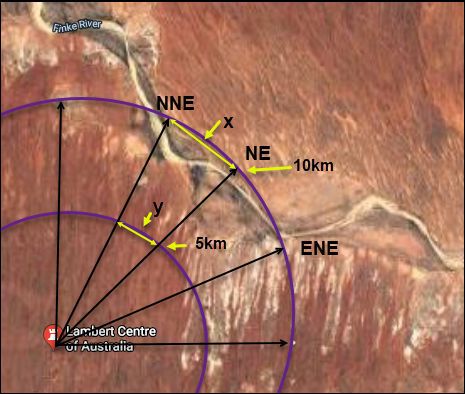
Using the example
10 km NE of Lambert Centre
and if we ignore distance imprecision, uncertainty due to the direction imprecision (Figure 11) is encompassed by an arc centered 10 km (d) from the center of Lambert Centre (at x,y) at a heading of 45 degrees (θ), extending 22.5 degrees in either direction from that point. At this scale the distance (e) from the center of the arc to the furthest extent of the arc (at x′,y′) at a heading of 22.5 degrees (θ′) from the center of Lambert Centre can be approximated by the Pythagorean Theorem,
where x=dcos(θ), y=dsin(θ), x′=dcos(θ′), and y′=dsin(θ′). The uncertainty in the above example would be 3.90 km.
This shows just one simple example. For details and formulae for calculating more complicated uncertainties, see Wieczorek 2001 and Wieczorek et al. 2004. Because of the complicated nature of these calculations, it is best to use the Georeferencing Calculator (Wieczorek & Wieczorek 2020) – see §3.4.9.
3.4.6. Uncertainty Related to Offset Precision
Precision can be difficult to gauge from a locality description as it is seldom, if ever, explicitly recorded. Further, a database record may not reflect, or may reflect incorrectly, the precision inherent in the original measurements, especially if the locality description in the database has undergone normalization, reformatting, or secondary interpretation of the original locality description.
There are a number of ways of calculating uncertainty from distances. In this document, we recommend a conservative approach, which assumes that many records have undergone a certain amount of interpretation or transformation when being entered into the database. Thus, a record of "10¼ mi" may be entered into the database as 10.25 mi. The precision implied in the value 10.25 is thus a false precision and the real precision should not be assumed to be between 10.24 and 10.26 or between 10.2 and 10.3. The method of Wieczorek et al. 2004, adapted here, bases the estimate of uncertainty on the fractional part of the distance, calculated by dividing 1 by the fractional denominator. The uncertainty would just be half of the precision. For example, 10.5 mi N of Bakersfield could reasonably be expected to mean 10½ mi with a precision of half a mile between 10.25 and 10.75 mi, or 10.5 with an uncertainty of 0.25 mi.
For distance measurements that are positive integer powers of 10, the precision should be ten to the next lower power. This calculation differs from Wieczorek et al. 2004, which recommended that the precision should be based on ten to the same power. Upon reconsideration, that seems excessive (see Table 5). This same reasoning can be used for precision in verbatim elevations and depths. Recommended values for uncertainty related to offset precisions are shown in Table 5.
Distance |
Recommended Uncertainty |
Uncertainty sec. Frazier et al. |
|---|---|---|
10.1 km |
0.05 km |
0.1 km |
10.25 mi |
0.125 mi |
0.01 mi |
10.5 km |
0.25 km |
0.1 km |
10.6 mi |
0.05 mi |
0.1 mi |
10.75 km |
0.125 km |
0.01 km |
10 mi |
0.5 mi |
1.5 mi |
15 km |
0.5 km |
1 km |
30 mi |
0.5 mi |
4.5 mi |
33 km |
0.5 km |
1 km |
100 mi |
5 mi |
15 mi |
140 km |
5 km |
21 km |
200 mi |
5 mi |
30 mi |
1000 m |
50 m |
150 m |
2000 m |
50 m |
300 m |
Precision can also be masked or lost when measurements are converted, such as from feet to meters, or from miles to kilometers.
| Be careful that the value you are using for precision when calculating the uncertainty is a true precision and not a false precision. For example, converting a collector’s recording of 16 miles (with a precision of 1 mile) to 25.6 km (with a precision of 0.1 km) leads to an unwarranted level of precision that is more than 16 times higher than the original. |
Figure 12 shows an example of two orthogonal distances measured from a feature, each with the uncertainty due to distance precision. If we ignore all sources of uncertainty except those arising from distance precision, the uncertainty is a bounding box centered on the point 8 km E and 6 km N of the corrected center of the feature. Each of the distance measurements demonstrates a precision of 1 km. Thus, each side of the box is a total of 1 km in length (0.5 km uncertainty in each cardinal direction from the center). Since we are characterizing the precision as a single distance measurement (1 km), we need the circle that circumscribes the above-mentioned bounding box to get the uncertainty due to the combined distance precisions. The radius of this circle is half the length of the distance precision bounding box, which is equal to one half the square root of two times the distance precision. So, for the above example the uncertainty associated with only the distance precision is one half the square root of two, or 0.707 km.
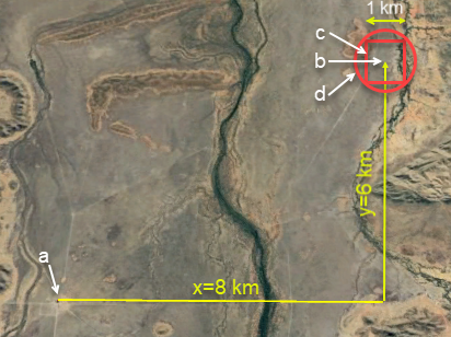
3.4.7. Combined Uncertainties
When combining uncertainties from different sources, it is not as simple as taking the average or adding them together. Uncertainties inherent in the location of the feature, in its extent, in the direction of the offset, and the distance of the offset, are just four sources that need to be combined to get an overall uncertainty. A detailed discussion of the calculations involved can be found in Wieczorek 2001 and Wieczorek et al. 2004. For a practical way of calculating uncertainties in locality descriptions, we recommend the Georeferencing Calculator (Wieczorek & Wieczorek 2020). To understand how each source of uncertainty contributes to the net overall uncertainty, see Understanding Uncertainty Contributions in the Georeferencing Calculator Manual (Bloom et al. 2020).
3.4.8. Using the Georeferencing Quick Reference Guide
The Georeferencing Quick Reference Guide (Zermoglio et al. 2020) is a practical guide for georeferencing giving step-by-step instructions on how to georeference a wide variety of locality types (see §3.2) following the best practices in this document and with specific reference on what to enter into the Georeferencing Calculator (Wieczorek & Wieczorek 2020).
3.4.9. Using the Georeferencing Calculator
The Georeferencing Calculator (Wieczorek & Wieczorek 2020) (Figure 13) is a tool to aid in georeferencing descriptive localities such as those found in museum-based natural history collections. It was originally designed for the Mammal Networked Information System (MaNIS) Project and has since been adopted by many other georeferencing initiatives. The current version and its Georeferencing Calculator Manual (Bloom et al. 2020) have been extensively upgraded to include new features and to bring it in line with this document.
The application makes calculations adapted from the methods originally described in the Georeferencing Guidelines (Wieczorek 2001) and later formalized in a peer-reviewed publication (Wieczorek 2004). We recommend its use generally by all natural history institutions to calculate uncertainty in location data without the need for a detailed understanding of the complicated underlying algorithms. The more institutions that use this one method, the more consistent will be the quality of data across and between institutions, making it easier for users to evaluate the quality of the data. We recommend reading both of the above-mentioned publications and the Georeferencing Calculator Manual (Bloom et al. 2020) for an understanding of the calculations involved and an understanding of how the Calculator works.
The Calculator can work online or locally in a browser (latest release available on GitHub). The source code is freely and openly available on GitHub.
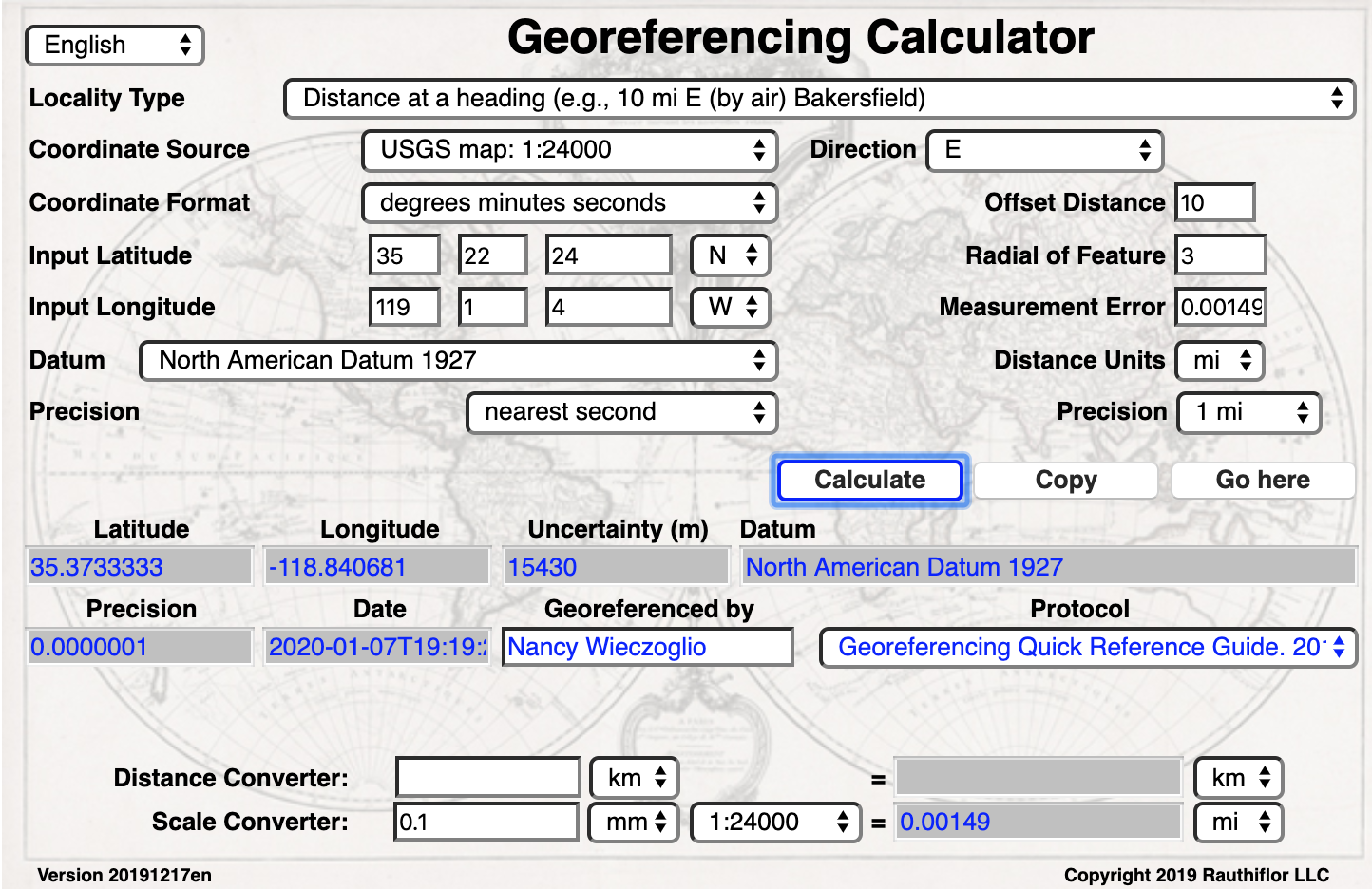
3.5. Difficult Localities
Some localities are difficult to georeference. For some the recommendation is to not even try. These are generally localities without sufficient information, with conflicting or ambiguous information, or where the information is explicitly in question. Some localities reference a feature that can’t be found with easily available resources. For these it may be just a matter of applying enough effort, but if the project is on a budget that can not support lengthy investigations into difficult localities, they may need to be left for another time. Difficult localities are not uncommon. Don’t despair. Some interesting ones have been documented by the MaNIS project.
Some marine localities can also provide difficulties – for example "Off Mar del Plata". The trouble is, one doesn’t know how far "off" Mar del Plata the event took place. In terrestrial localities one can generally make a decision that it is between the feature and the next feature, but in the marine environment, that may not be as easy. Does it mean "within sight of", 5km, 12km, the EEZ boundary, the continental shelf…? One does not reliably know the end point so it makes it difficult (if not impossible) to georeference accurately. One good resource for finding marine localities, boundaries, etc. is the website marineregions.org (VLIZ 2019).
3.6. Determining Spatial Fit
Spatial fit, first formalized as the Reock degree of compactness (Young 1988, Reock 1961), is a georeferencing concept designed to measure how well a given geometric representation matches the original spatial representation. This is useful when spatial transformations change the way a locality is represented, either to mask its detail, or to match an agreed upon schema for data sharing (such as fitting locations to a grid cell).
A spatial fit with a value of "1" is an exact match or 100 per cent overlap. If the geometry given does not completely encompass the original spatial representation, then the spatial fit is zero (i.e. some of the original is outside the transformed version, which we interpret as not being a fit). If the transformed shape does completely encompass the original spatial representation, then the value of the spatial fit is the ratio of the area of the transformed geometry to the area of the original spatial representation. Special case: If the original spatial representation is a point and the geometry presented is not a point, then the spatial fit is undefined. The range of values of spatial fit is 0, 1, greater than 1, or undefined (see Figure 14 and Table 6, Table 7, Table 8 and Table 9).
An example of the applicability of the spatial fit is where a point representing a terrestrial collection lies close to the coast, and the calculated uncertainty radius encompasses some marine area. In this case the spatial fit would be greater than 1 as it represents an area greater than the real uncertainty (Figure 15). Spatial fit is also a valuable measure for describing the degree of generalization of a sensitive species, for example see §5.2 and Chapman 2020.
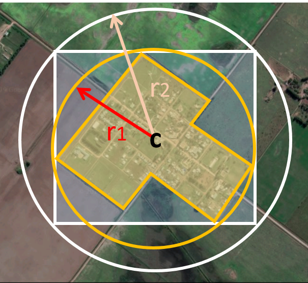
Figure 14 illustrates a few examples of the definition of spatial fit and these are elaborated in the Tables below:
The spatial fit of the white circle (r₂) |
\$(pi r_2^2)/A\$ |
The spatial fit of the bounding box |
\$(2 r_2^2)/A\$ |
The spatial fit of the yellow circle (r₁) |
\$(pi r_1^2)/A\$ |
The spatial fit of the polygon |
1 |
The spatial fit of the point C |
0 |
The spatial fit of the white circle (r₂) |
\$(pi r_2^2)/(2r_2^2)\$ |
The spatial fit of the bounding box |
1 |
The spatial fit of the yellow circle (r₁) |
0 |
The spatial fit of the polygon |
0 |
The spatial fit of the point C |
0 |
The spatial fit of the white circle (r₂) |
\$r_2^2/r_1^2\$ |
The spatial fit of the bounding box |
0 |
The spatial fit of the yellow circle (r1) |
1 |
The spatial fit of the polygon |
0 |
The spatial fit of the point C |
0 |
The spatial fit of the white circle (r2) |
Undefined |
The spatial fit of the bounding box |
Undefined |
The spatial fit of the yellow circle (r1) |
Undefined |
The spatial fit of the polygon |
Undefined |
The spatial fit of the point C |
1 |
Figure 15 shows an example of applying the spatial-fit concept of a point-radius method of describing uncertainty where it is restricted to a shape method representation. For example, the location of a plant along the coast of north-east Madagascar – marked with the yellow X (Figure 15) – has an uncertainty radius of approx 1.35 km, but we know the record is of a terrestrial plant species so we can calculate the true area of uncertainty by excluding the marine biome using the shape method, thus the spatial fit is the ratio of the area of the red circle (5.726 sq km) divided by the area of the blue shaded area (~4.1 sq km) giving a spatial fit of the uncertainty radius of 1.39.
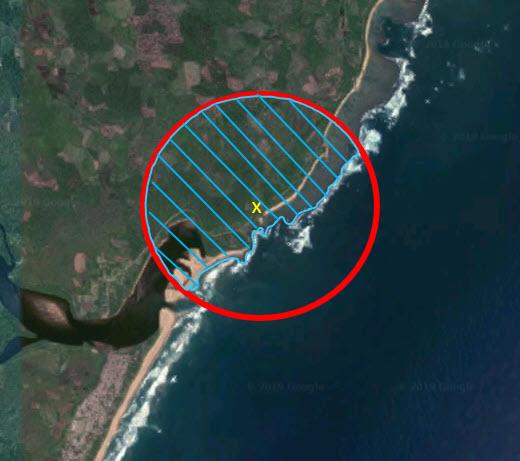
4. Collaborative Georeferencing
The characteristics that make a georeferencing project collaborative are the aggregation of occurrence records from multiple participating groups (e.g. datasets, collections, institutions), the extraction of distinct localities as the actual target of georeferencing, the standardization of the geography of the aggregated records to aid record grouping and assignment by geography.
Collaborative georeferencing, if done properly, can have definitive advantages over georeferencing alone. MaNIS (Wieczorek 2001) and Australia’s Virtual Herbarium (ANBG 2018) found that collaborative georeferencing resulted in great efficiency gains, but that including validation checks afterwards by reviewing the records using collector and date, or looking at the records taxonomically to check for outliers, and other such data quality flags, is important. Advantages and disadvantages of collaborative georeferencing, adapted from Wieczorek & Beaman 2002 and Stein & Wieczorek 2004 include:
Advantages
-
Reduces overall cost of supplies (e.g. maps) – no duplication.
-
Expands the pool of resources – geographic expertise and reference materials.
-
Takes advantage of regional expertise, knowledge, language skills and resources.
-
Increases georeferencing rates – economy of scale.
-
Promotes standardization of methods.
-
Increases skills in a community.
-
Increases exposure and awareness inside and outside of a community - strengthens community relationships.
Disadvantages
-
Vulnerable to procrastination, delays, uneven levels of training, expertise and commitment.
-
Can distance the georeferencing process from useful primary resources (e.g. specimen labels and field notes).
-
Introduces time sensitivity to the georeferencing process (locality information for the underlying occurrence records might be subject to changes during the georeferencing process that would render a different result).
-
Data repatriation into the originating collection can be a difficult and time-consuming process.
-
Requires project-level management.
-
Requires a formalized validation process.
One of the greatest impediments to effective collaborative georeferencing is the absence of tools to easily repatriate the georeferenced information back to the data sources (Barkwell and Murrell 2012, Grant et al. 2018). A number of projects are working on this, especially §4.3 in conjunction with the Symbiota platform (Gries et al. 2014). It is hoped that this document will provide consistency of methodology and documentation and lead to more collaborative georeferencing.
Some organizations, such as DigiVol (Australian Museum n.d.) and Notes from Nature (Zooniverse n.d.) use crowdsourcing to georeference, whereas projects like CoGeo (part of GEOLocate, GEOLocate 2018), are more constrained in their participants.
4.1. DigiVol
The Atlas of Living Australia, in collaboration with the Australian Museum, developed DigiVol (Australian Museum n.d.) to harness the power of online volunteers (also known as crowdsourcing) to digitize biodiversity data that is locked up in biodiversity collections, field notebooks and survey sheets. Although originally developed in Australia, DigiVol has many projects and expeditions from all over the globe. Not all DigiVol projects (called expeditions) include a georeferencing component, but some of them do, and there is no reason that there won’t be more in the future.
The Australian Museum has developed a guide for a mapping tool to use with DigiVol (Edey n.d.). The mapping tool, however, has a number of features that we would not recommend. Default positions are given for the "center" of a number of Australian States without an appropriate associated uncertainty value. The uncertainty of the georeference is added by a pulldown menu that gives three options: 1km, 5km and 10km. Our recommendation would be to make uncertainty continuous–possibly by selection on the map, or calculated using the body of information in this document, the protocols of the Georeferencing Quick Reference Guide (Zermoglio et al. 2020), and the algorithms of the Georeferencing Calculator (Wieczorek & Wieczorek 2020).
4.2. Notes from Nature
The Notes from Nature project (Zooniverse n.d.) gives people the opportunity to make scientifically important contributions toward the goal of conserving and making available knowledge about natural and cultural heritage. "Every transcription that is completed brings us closer to filling gaps in our knowledge of global biodiversity and natural heritage". It is very similar to DigiVol. Currently, there are no georeferencing projects (expeditions) in Notes from Nature, but there are plans to develop this in the future.
4.3. GEOLocate
The GEOLocate suite of tools includes a web-based collaborative client – CoGeo (Rios 2019), the goal of which is to provide a mechanism whereby groups of users can form communities to collaboratively georeference and verify a shared dataset (GEOLocate 2018). This allows for the upload of a CSV file and having parts of the dataset allocated to a user. GEOLocate can also be accessed through third party applications via its API.
Using the tools in GEOLocate, a georeference may be determined along with an uncertainty (Biedron & Famoso 2016). An uncertainty polygon (see also shape and §3.3.4) can also be drawn in addition to the point-radius circle. Note that GEOLocate may return more than one candidate location for a given locality string and users are advised to always verify and adjust, as needed, to obtain the final accepted result (including uncertainty radii and polygons). The data can be exported through KML for plotting onto Google Earth. The system allows for review of records and we recommend that this be done for all records where possible.
4.4. Other Collaborative Georeferencing Projects
Other projects, including the terrestrial vertebrate precursor projects to VertNet (Stein & Wieczorek 2004, Guralnick & Constable 2010), have, in the past, divided up and distributed the records for localities from a given geographic region to an institution with expertise in and/or resources about that region to georeference (see §3.1.2). The major advantages of this approach are that the quantity and quality of the raw materials used for georeferencing are probably higher, and the efficiency and quality of the results are also likely higher than if attempted without taking advantage of these resources. However, as mentioned earlier, repatriation of the georeferenced records is an issue that needs solving for this to work most efficiently.
5. Sharing Data
Georeferencing is only the first step toward making biological (specimen and observation) data available to the world. However, it is an important first step, as it is one of the two most key methods for identifying what and where a specimen is, that is, its scientific name and its location (Chapman 2005a). Two main standards have been developed for sharing biological data, Darwin Core (Wieczorek et al. 2012b) and Access to Biological Collections Data (ABCD), both ratified by Biodiversity Information Standards (TDWG). We do not treat the ABCD standard separately in this document, as term mappings between Darwin Core and ABCD are well defined for location data. One of the principles of Darwin Core is to try to provide content for every field possible.
5.1. Mapping to Darwin Core
The Darwin Core (denoted with the abbreviated namespace dwc) georeferencing concepts that are directly used in this document are:
- dwc:decimalLatitude, dwc:decimalLongitude
-
the geographic coordinates of the center of the point-radius version of the georeference
- dwc:geodeticDatum
-
the EPSG code (preferably) or name of the coordinate reference system, geodetic datum, or ellipsoid of the point-radius version of the georeference
- dwc:coordinateUncertaintyInMeters
-
the radial of the point-radius version of the uncertainty of the georeference, in meters
- dwc:coordinatePrecision
-
the decimal representation of the precision of the output coordinates of the georeference
- dwc:footprintWKT
-
the representation of the resulting shape or bounding box georeference, in Well-Known Text (WKT) (ISO 2016)
- dwc:footprintSRS
-
the coordinate reference system of the resulting shape or bounding box georeference, in Well-Known Text (WKT) (ISO 2016)
- dwc:locality
-
intended to contain a version (perhaps modified from the original) of the parts of the textual description of the location that do not have another Darwin Core term appropriate to hold them; in legacy data, may contain any textual information about the location
- dwc:verbatimLocality
-
meant to contain all of the unmodified original location information
- dwc:verbatimCoordinates
-
the original coordinates in the original format, especially if they are not latitude and longitude, such as Universal Transverse Mercator (UTM) coordinates
- dwc:verbatimLatitude, dwc:verbatimLongitude
- dwc:verbatimCoordinateSystem
-
the coordinate format of the coordinates that are either in dwc:verbatimCoordinates or in dwc:verbatimLatitude and dwc:verbatimLongitude
- dwc:verbatimSRS
-
the coordinate reference system of either the dwc:verbatimCoordinates or the combination of dwc:verbatimLatitude and dwc:verbatimLongitude
- dwc:minimumElevationInMeters, dwc:maximumElevationInMeters
-
the lower and upper limits of the elevation of the location, in meters
- dwc:verbatimElevation
-
the original elevation in the original format with the original units
- dwc:minimumDepthInMeters, dwc:maximumDepthInMeters
-
the minimum and maximum limits of the depth of the location, in meters
- dwc:verbatimDepth
-
the original depth in the original format with the original units
- dwc:minimumDistanceAboveSurfaceInMeters, dwc:maximumDistanceAboveSurfaceInMeters
-
the lower and upper limits of the position with respect to a local surface, either at an elevation, or at a depth from an elevation.
- dwc:locationAccordingTo
-
the source authority for the location information, not the georeference information, for which see dwc:georeferenceSources
- dwc:locationRemarks
-
comments about the location information, not about the georeference for the location, for which see dwc:georeferenceRemarks
- dwc:pointRadiusSpatialFit
-
the spatial fit of the point-radius georeference (see §3.6)
- dwc:footprintSpatialFit
-
the spatial fit of the shape or bounding box georeference (see §3.6)
- dwc:georeferencedBy
-
who is responsible for the georeference as it currently stands, could be the person who did the first pass, but could be changed later to the person who verifies it
- dwc:georeferencedDate
-
the date on which the data in the georeference fields reached their current state
- dwc:georeferenceProtocol
-
a citation of a published set of rules used to determine a georeference. For example, “Georeferencing Quick Reference Guide 2020”. Any deviations from the cited protocol should be noted in dwc:georeferenceRemarks
- dwc:georeferenceSources
-
a list of maps, gazetteers, or other resources used to georeference the locality. Should be specific enough that someone else can locate and use the same sources. Example: "USGS 1:24000 Florence Montana Quad 1967; Terrametrics 2008, Google Earth".
- dwc:georeferenceVerificationStatus
-
an indicator of the extent to which the georeference has been verified to represent the best possible spatial description for the occurrence record. By default a newly created georeference should have the status "requires verification". Beyond that, there are really only two other functionally distinct possibilities, either "verified" (by the person mentioned in dwc:georeferencedBy), and "verified by collector" or equivalent, to designate that the georeference was reviewed for that specific record by the person who recorded it to begin with, and that it can not be further improved. This is the ideal status to aspire to.
- dwc:georeferenceRemarks
-
any notes or comments about the spatial description, deviations from the cited protocol, assumptions, or problems with georeferencing. For example, "locality too vague to georeference".
5.2. Generalizing Georeferences for Sensitive Taxa and Locations
As recommended elsewhere in this document, georeferences should be recorded and stored at the best possible resolution and precision. If, however, the location of a taxon is regarded as sensitive for some reason following the guidelines as set out in Chapman 2020 and Chapman & Grafton 2008, and it is agreed that the detailed location information should not be shared, we recommend, that the data only be generalized at the time of sharing or publishing of the data.
We recommend that if data are to be generalized that it be done by reducing the number of decimal places (for example when using decimal degrees) at which the data are published (Chapman & Grafton 2008, Chapman 2020). Good practice dictates that whatever you do to generalize the data, it be documented so that users of the data know what reliance can be placed on them. As far as the generalization of georeferencing data is concerned it is important to record that the data have been generalized using a ‘decimal geographic grid’, and record both:
-
Precision of the data provided (e.g. 0.1 degree; 0.001 degree, etc.)
-
Precision of the data stored or held (e.g. 0.0001 degree, 0.1 minute, 1 second, etc.)
We recommend that when recording the degree of generalization of data, that Spatial Fit (§3.6) be used. For example, the degree to which a record has been generalized to obfuscate the georeference will be a number greater than 1 (see Figure 14 and Chapman 2020).
| Data should never be generalized at the time of collection, when georeferencing or when storing in the database. |
Some institutions randomize the data before publishing. This is a practice we do NOT recommend, and in fact would discourage it in all circumstances (Chapman 2020).
6. Maintaining Data Quality
Data that have been incorporated into the database and georeferenced need to be maintained and checked for quality. The quality checking process involves a number of steps, including receiving feedback from users, providing feedback to collectors, and running various validation tests. For more information on data quality and what it means for primary species collection data, see Chapman 2005c. Two major principles associated with data quality and data cleaning are:
-
Error prevention is preferable to error correction.
-
The earlier in the information chain that you can detect an error, the cheaper it will be to correct it.
6.1. Feedback to Collectors
Improving the quality of the data may require giving feedback to others. For example, if you find that a particular collector is not recording his collection information correctly (e.g. not recording the datum with the coordinate information), then you need to provide feedback so that future records have a lower level of uncertainty and thus a higher quality. See the earlier chapter on §2. Key issues that may require feedback to collectors include:
-
Making sure the datum or coordinate reference system is recorded with all GPS readings
-
Encouraging consistent use of a standard coordinate format (e.g. encourage collectors to use decimal degrees wherever possible)
-
Recording localities in a consistent and clear manner:
-
Ensure that they document all their processes and methodologies for recording locality and locality-associated information such as elevation
-
Encourage training in, and the adoption of, best practices such as laid out in this document
6.2. Accepting Feedback from Users
Feedback from users can be one of the most valuable resources for improving the quality of one’s collections and observations. For this to work, however, the institution needs to set up a good feedback mechanism. There needs to be a process whereby all feedback related to quality are checked and the results documented (see Chapman 2005a & Chapman 2005b). Feedback may be from other institutions holding duplicates of specimens, from users who are carrying out analyses on large amounts of data and find records that are either wrongly georeferenced, or wrongly identified, or from users who are carrying out data quality checking on related records. All feedback is important, and should not be ignored. Checks carried out should also always be documented so that the same ‘error’ is not checked over and over again, for example, with dwc:georeferenceVerificationStatus. Having a unique way to reference specimens can be important, and makes feedback much more efficient (see §1.9).
6.3. Data Checking and Cleaning
An important but often overlooked aspect to any georeferencing project is the checking of the georeferenced data that goes into the database. This aspect is often ignored because of lack of funds or personnel. However, because the point of any georeferencing project is to produce geographic coordinates linking a specimen or observation to a place on a map or to environmental data, it is important that the coordinates chosen are truly the best ones for the location. Not only does it improve the quality of data, but it also identifies trends and habits in georeferencing that may need to be corrected.
6.3.1. Data Entry
One of the major sources of error in georeferencing is at the stage of data entry. Errors can be reduced by the establishment of good data entry procedures – use of pick lists, field constraints, etc. Many of these issues should also be addressed as part of the database design (see §3.1.1.4). Good database design can reduce many of the errors associated with data entry. However, once these are in place and working, then regular checks need to be carried out on the data entry operators and on the process of data entry.
One method developed for the MaPSTeDI project (Murphy et al. 2004) is to first check the accuracy of the georeferencing. This process involves checking a certain number of each georeferencer’s records. Based on various trials, it is recommended that the first 200 records that a new georeferencer completes be checked for accuracy. Not only is this initial checking beneficial to the accuracy of the data, but also it is essential to allow the georeferencer to improve and learn through feedback from making mistakes. We recommend the following protocol for checking data quality:
-
Check the initial 200 records. If problems remain, check groups of 100 until satisfied with the georeferencer’s abilities.
-
Regularly check 10 randomly selected records out of every 100.
-
If there are more than two incorrect records, the quality checker should check 20 more records and can ask the georeferencer to redo the entire 100.
-
After a while, the regular checks can be reduced to five records out of every 100.
The second purpose of quality checking is to allow georeferencers to refer difficult or confusing records to the quality checker for help or advice. The quality checker will then resolve these ‘problem records’ as well as possible. Checking problem records can be like detective work. Historical records often have locality descriptions with features that do not appear on modern maps or in gazetteers. To find these localities, it is often necessary to consult several different sources of information. These sources include, but are not limited to catalogue books, field notes, other records with similar localities, other collections, scientific and other publications, websites, online databases, speciality gazetteers, and historical maps. Bits of information from several places can often be used to establish the correct coordinates for a historical locality.
In addition, some problem records do not make sense because of contradictions or missing or garbled information. These problem records may be the result of mistakes in data entry made in either the paper catalogue or the database. It may also be necessary to consult the curatorial staff or even the original collector. If georeferencing information is able to be found for difficult locations, then it is worthwhile documenting them for future use, or even publishing the results of your searches, as seldom are unusual localities orphans and you, or others, may come across the same locality again at a later date.
6.3.2. Data Validation
Data validation (checking for errors) can be a time-consuming process; however, it is one of the most important processes you can carry out with your data. It is not practical to check every record individually, so the use of batch processing techniques and outlier detection procedures, etc., is essential. Fortunately, a number of these have been developed and are available in software products or online (see georeferencing.org and Chapman 2005b). The information in those resources are not repeated here. We recommend that you incorporate some of those methodologies into your own working practices.
There are many methods of checking for errors in georeferenced data. These can involve:
-
Using external databases (collectors’ itineraries, gazetteers, etc.)
-
Checking against other fields in your own database (making sure the georeference falls within the correct state, country, region, etc.)
-
Using a GIS to look for records that fall outside polygon boundaries such as bioregions, local government areas, terrestrial/aquatic/marine areas
-
Using statistical methods such as box plots, reverse jackknifing, cumulative frequency curves and cluster analysis to identify outliers in latitude and longitude or elevation
-
Using expert-derived range maps
-
Using taxon lists – for example, using a list of marine taxa to determine if a record should be marine or not, and similarly with terrestrial and freshwater aquatic taxa
-
Using modelling software in conjunction with statistical analysis to identify outliers in environmental (e.g. climate) space
Some of these techniques are incorporated into a number of programs including Biogeo (Robertson et al. 2016), CoordinateCleaner (Zizka et al. 2019) and the stand-alone GIS software DIVA-GIS (Hijmans et al. 2012). See also georeferencing.org.
The Data Quality Interest Group of TDWG established a Task Group in 2014 to develop a set of Core Tests and Assertions for checking and validating the quality of species occurrence data (specimens and observation, etc.). The resulting 101 tests based on Darwin Core terms will be coded and available for use in 2020 (Chapman et al. 2020). Currently (as of February 2020), there are 12 validation tests related to coordinates and datums and another seven related to geography. In addition there are seven amendment tests that can be used to improve the quality of the data.
6.3.3. Making Corrections
When making corrections to your database, we strongly recommend that you always add and never replace or delete. For this to happen you will usually require additional fields in the database. For example, you may have ‘original’ or ‘verbatim’ georeference fields in addition to the main georeference fields. Additionally, the database may require a number of ‘Remarks/Notes/Comments’ fields. Fields that can be valuable are those that describe validation checking that has been carried out – even (and often especially) if that checking has led to confirmation of the georeference. These fields may include information on what checks were carried out, by whom, when and with what results. Be sure to update the equivalent of dwc:georeferenceVerificationStatus and associated fields (dwc:georeferencedBy, dwc:georeferencedDate) whenever changes are made to the georeference.
6.4. Responsibilities of the Manager
It is important that the manager maintain good sets of documentation (guidelines, best practice documents, etc.), ensure that there are effective feedback mechanisms in place, and ensure that up-to-date data quality procedures are being implemented. For further responsibilities, we refer you to the document Principles of Data Quality (Chapman 2005a), which should be read as an adjunct to this document.
6.5. Responsibilities of the Supervisor
The georeferencing supervisor has the principle responsibility for monitoring and maintaining the quality of the data on a day-to-day basis. Perhaps their key responsibility is to supervise the data-entry procedures (see §6.3.1), and the data validation, checking and cleaning processes. This role is key in any georeferencing process, along with that of the data entry operators. It is important that the duties and responsibilities be documented in the institution’s best practice manuals and guidelines.
6.6. Training
Training is a major responsibility of anyone beginning or conducting the georeferencing. Good training can reduce the level of error, reduce costs, and improve data quality.
Topics of a five day course may include (depending on the audience, and not in this order) the following, adapted from Paul 2018:
-
Introduction to georeferencing
-
Developing a georeferencing project
-
Georeferencing best practices
-
Georeferencing Quick Reference Guide (Zermoglio et al. 2020)
-
Using the Georeferencing Calculator (Wieczorek & Wieczorek 2020)
-
Geographic concepts
-
Good and bad localities
-
Using gazetteers
-
Using physical maps
-
Using Google Earth and Google Maps
-
Recording uncertainty using the point-radius method
-
Using the shape method of georeferencing uncertainty
-
Using online tools
-
Finding Internet resources
-
From collaboration to automation
-
Reporting through Darwin Core
-
Validating georeferences.
-
Repatriating data
-
Building end-to-end georeferencing workflows
-
Sharing georeferenced data
| Georeferencing training has a learning curve that in some cases can be steep. As a good georeferencing practice involves having knowledge of several different areas (e.g. geography, informatics, biodiversity data, data standards, etc.), make sure to establish a solid selection process of the participants. This will help you reduce the time and resources needed for training and, more importantly, will reduce the probability of errors and improve the quality of the data. |
6.7. Performance Criteria
The development of performance criteria is a good way of ensuring a high level of effectiveness, efficiency, consistency, accuracy, reliability, transparency, and quality in the database. Performance criteria can relate to an individual (data entry operator, supervisor, etc.) or to the process as a whole. It can relate to the number of records entered per unit time, but we would recommend that it should relate more to the quality of entry — some locality types and some geographic regions are simply more difficult than others. Where possible, performance criteria should be finite and numeric so that performance against the criteria can be documented. Some examples may include:
-
90 per cent of records will undergo validation checks within 6 months of entry.
-
Any suspect records identified during the validation procedures will be checked and corrected within 30 working days.
-
Feedback from users on errors will be checked and the user notified of the results within two weeks.
-
All documentation of validation checks will be completed and up-to-date.
-
Updated data will be published on a monthly basis.
6.8. Index of Spatial Uncertainty
An Index of Spatial Uncertainty may be developed and documented for the dataset as a whole to allow for overall reporting of the quality of the dataset. This index would supplement a similar index of other data in the database, such as an index of Taxonomic Uncertainty and would generally be for internal use, but may be shared as part of an institution’s metadata. Currently, no such universal index exists for primary species occurrence data, but institutions may consider developing their own and testing its usefulness. Such indexes should, wherever possible, be generated automatically and produced as part of a data request from the database and packaged with the metadata as part of the request. Such an index could form the basis for helping users determine the quality of the database for their particular use. The authors of this document would be interested in any feedback from institutions that develop such an index. The index should form an integral part of the metadata for the dataset and may include the following for the georeferencing part of the database:
-
Completeness Index
-
Percentage of records with minimum recommended georeference fields that have valid values
-
Percentage of records with an extent field that has a value
-
Percentage of records with an uncertainty field that has a value
-
Percentage of records with a coordinate precision field that has a value
-
Percentage of records with datum fields that have a known datum or coordinate reference system value
-
-
Uncertainty Index
-
Average and standard deviation of ‘uncertainty’ value for those records that have a value.
-
Percentage of records with a maximum uncertainty distance value in each class:
-
<100 m
-
100-1,000 m
-
1,000-2,000 m
-
2,000-5,000 m
-
5,000-10,000 m
-
>10,000 m
-
Not determined
-
-
-
Currency Index
-
Time since last data entry
-
Time since last validation check
-
-
Validation Index
-
Percentage of records that have undergone validation test x
-
Percentage of records that have undergone validation test y, etc.
-
Percentage of records identified as suspect using validation tests
-
Percentage of suspect records found to be actual errors
-
The tests arising from the TDWG Data Quality Interest Group include 4 Measure tests at the record level (Chapman et al. 2020):
-
Number of Validation tests where prerequisites were not met
-
Number of Validation tests that were compliant
-
Number of Validation tests that were not compliant
-
Number of Amendments proposed
6.9. Documentation
Documentation is one of the key aspects of any georeferencing process. Documentation involves everything from record-level documentation such as:
-
How the georeference was determined
-
What method was used to determine the radial and uncertainty
-
What modifications were made (for example, if an operator edits a point on the screen and moves it from point ‘a’ to point ‘b’ it is best practice to document "why" the point was moved and not just record that location was moved from point ‘a’ to point ‘b’ by the operator)
-
Any validation checks that were carried out, by whom and when
-
Flags that may indicate uncertainty, etc.
Documentation also includes the metadata related to the collection as a whole, which may include:
-
The overall level of data quality
-
The general checks carried out on the whole dataset
-
The units of measurement and other standards adopted
-
The guidelines followed
-
The §6.8 (see earlier discussion, this section)
A second set of documentation relates to:
-
The institution’s ‘Best Practice’ document which we recommend should be derived from this document and tailored to the specific needs of the institution
-
Training manuals
-
Standard database documentation
-
Guidelines and standards
We recommend that documentation be made an integral part of any georeferencing process.
6.9.1. Truth in Labelling
‘Truth in Labelling’ is an important consideration with respect to documenting data quality. This is especially so where data are being made available to a wider audience, for example, through GBIF. We recommend that documentation of the data and their quality be upfront and honest. Error is an inescapable characteristic of any dataset, and it should be recognized as a fundamental attribute of those data. All databases have errors, and it is in no one’s interest to hide those errors (Chrisman 1991). On the contrary, revealing data actually exposes them to editing, validation and correction through user feedback, while hiding information almost guarantees that it will remain dirty and of little long-term value.
Glossary
The purpose of this glossary is to describe important concepts in accordance with the intended meaning in this document, the associated Georeferencing Quick Reference Guide (Zermoglio et al. 2020) and the Georeferencing Calculator Manual (Bloom et al. 2020). These concepts are treated in broader contexts in many other sources. We have adapted the terms presented here from many sources including Wikipedia (as of November 2019), the ESRI Dictionary (as of November, 2019) (ESRI n.d.), and various articles within Kemp 2008.
- accuracy
-
The closeness of an estimated value (for example, measured or computed) to a standard or accepted ("true") value. Antonym: inaccuracy. Compare error, bias, precision, false precision and uncertainty.
"The true value is not known, but only estimated, the accuracy of the measured quantity is also unknown. Therefore, accuracy of coordinate information can only be estimated." (Geodetic Survey Division 1996, FGDC 1998). - altitude
-
A measurement of the vertical distance above a vertical datum, usually mean sea level or geoid. For points on the surface of the Earth, altitude is synonymous with elevation.
- antimeridian
-
The meridian of longitude opposite a given meridian. A meridian and its antimeridian form a continuous ring around the Earth. The "Antimeridian" is the specific meridian of longitude opposite the prime meridian and is used as the rough basis of the International Date Line.
- bathymetry
-
-
The measure of depth of water in oceans, seas and lakes.
-
The shapes of underwater terrains, including underwater topography and sea floor mapping.
-
- bias
-
The difference between the average value of a set of measurements and the accepted true value. Bias is equivalent to the average systematic error in a set of measurements and a correction to negate the systematic error can be made by adjusting for the bias. Compare accuracy, error, precision, false precision and uncertainty.
- boundary
-
The spatial divide between what is inside a location and what is outside of it.
- bounding box
-
An area defined by the coordinates of two diagonally opposite corners of a polygon, where those two corners define the north-south and east-west extremes of the area contained within.
- clause
-
see locality clause.
- coordinate format
-
The format in which coordinates are encoded, such as "decimal degrees", "degrees minutes seconds", "degrees decimal minutes", or Universal Transverse Mercator (UTM).
- coordinate precision
-
The fraction of a degree corresponding to the number of significant digits in the source coordinates. For example, if the coordinates are reported to the nearest minute, the precision is 1/3600th (0.00027778) of a degree; if a decimal degree is reported to two decimal places, the precision is 0.01 of a degree.
- coordinate reference system
-
(also spatial reference system) A coordinate system defined in relation to a standard reference or datum.
- coordinate system
-
A geometric system that defines the nature and relationship of the coordinates it uses to uniquely define positions. Examples include the geographic coordinate system and the Universal Transverse Mercator (UTM) coordinate system.
- coordinate uncertainty
-
A measure of the minimum distance on the surface from a coordinate within which a locality might be interpreted to be.
- coordinates
-
A set of values that define a position within a coordinate system. Coordinates are used to represent locations in space relative to other locations.
- coordinateUncertaintyInMeters
-
The Darwin Core term corresponding to the maximum uncertainty distance when given in meters.
- corrected center
-
The point within a location, or on its boundary, that minimizes the geographic radial of the location. This point is obtained by making the smallest enclosing circle that contains the entire feature, and then taking the center of that circle. If that center does not fall inside the boundaries of the feature, make the smallest enclosing circle that has its center on the boundary of the feature. Note that in the second case, the new circle, and hence the radial, will always be larger than the uncorrected one (see Figure 4).
- Darwin Core
-
A standard for exchanging information about biological diversity (see Darwin Core).
- data quality
-
‘Fitness for use’ of data (Juran 1964, Juran 1995, Chrisman 1991, Chapman 2005a). As the collector of the original data, you may have an intended use for the data you collect but data have the potential to be used in unforeseen ways; therefore, the value of your data is directly related to the fitness of those data for a variety of uses. As data become more accessible, many more uses become apparent (Chapman 2005c).
- datum
-
A set of one or more parameters that serve as a reference or basis for the calculation of other parameters ISO 19111. A datum defines the position of the origin, the scale, and the orientation of the axes of a coordinate system. For georeferencing purposes, a datum may be a geodetic datum or a vertical datum.
- decimal degrees
-
Degrees expressed as a single real number (e.g. −22.343456). Note that latitudes south of the equator are negative, as are longitudes west of the prime meridian to −180 degrees. See also decimal latitude and decimal longitude.
- decimal latitude
-
Latitude expressed in decimal degrees. The limits of decimal latitude are −90 to 90, inclusive.
- decimal longitude
-
Longitude expressed in decimal degrees. The limits of decimal longitude are −180 to 180, inclusive.
- declination
-
see magnetic declination.
- DEM
- depth
-
A measurement of the vertical distance below a vertical datum. In this document, we try to modify the term to signify the medium in which the measurement is made. Thus, "water depth" is the vertical distance below an air-water interface in a waterbody (ocean, lake, river, sinkhole, etc.). Compare distance above surface. Depth is always a non-negative number.
- digital elevation model (DEM)
-
A digital representation of the elevation of locations on the surface of the earth, usually represented in the form of a rectangular grid (raster) that stores the elevation relative to mean sea level or some other known vertical datum. The term Digital Terrain Model (DTM) is sometimes used interchangeably with DEM, although it is usually restricted to models representing landscapes. A DTM usually contains additional surface information such as peaks and breaks in slope.
- direction
-
see heading.
- distance above surface
-
In addition to elevation and depth, a measurement of the vertical distance above a reference point, with a minimum and a maximum distance to cover a range. For surface terrestrial locations, the reference point should be the elevation at ground level. Over a body of water (ocean, sea, lake, river, glacier, etc.), the reference point for aerial locations should be the elevation of the air-water interface, while the reference point for sub-surface benthic locations should be the interface between the water and the substrate. Locations within a water body should use depth rather than a negative distance above surface. Distances above a reference point should be expressed as positive numbers, while those below should be negative. The maximum distance above a surface will always be a number greater than or equal to the minimum distance above the surface. Since distances below a surface are negative numbers, the maximum distance will always be a number less than or equal to the minimum distance. Compare altitude.
- DMS
-
Degrees, minutes and seconds – one of the most common formats for expressing geographic coordinates on maps. A degree is divided into 60 minutes of arc and each minute is divided into 60 seconds of arc. Degrees, minutes and seconds are denoted by the symbols °, ′, ″. Degrees of latitude are integers between 0 and 90, and should be followed by an indicator for the hemisphere (e.g. N or S). Degrees of longitude are integers between 0 and 180, and should be followed by an indicator for the hemisphere (e.g. E or W).
- easting
-
Within a coordinate reference system (e.g. as provided by a GPS or a map grid reference system), the line representing eastward distance from a reference meridian on a map.
- elevation
-
A measurement of the vertical distance of a land or water surface above a vertical datum. On maps, the reference datum is generally some interpretation of mean sea level or the geoid, while in devices using GPS/GNSS, the reference datum is the ellipsoid of the geodetic datum to which the GPS unit is configured, though the device may make corrections to report the elevation above mean sea level or the geoid. Elevations that are above a reference point should be expressed as positive numbers, while those below should be negative. Compare depth, distance above surface, and altitude.
- ellipsoid
-
A three-dimensional, closed geometric shape, all planar sections of which are ellipses or circles. An ellipsoid has three independent axes. If an ellipsoid is made by rotating an ellipse about one of its axes, then two axes of the ellipsoid are the same, and it is called an ellipsoid of revolution. When used to represent a model of the earth, the ellipsoid is an oblate ellipsoid of revolution made by rotating an ellipse about its minor axis.
- entry point
-
The entry point on the surface of the ocean or lake where a diver enters the water and from which all activities are measured. See Figure 7.
- EPSG
-
EPSG codes are defined by the International Association of Oil and Gas Producers, using a spatial reference identifier (SRID) to reference spatial reference systems. The EPSG Geodetic Parameter Dataset (IOPG 2019) is a collection of definitions of coordinate reference systems (including datums) and coordinate transformations which may be global, regional, national or local in application.
- error
-
The difference between a computed, estimated, or measured value and the accepted true, specified, or theoretically correct value. It encompasses both the imprecision of a measurement and its inaccuracies. Error can be either random or systematic. If the error is systematic, it is called "bias". Compare accuracy, bias, precision, false precision and uncertainty.
- event
-
A process occurring at a particular location during a period of time. Used generically to cover various kinds of collecting events, sampling events, and observations.
- extent
-
The entire space within the boundary a location actually represents. The extent can be a volume, an area, or a distance.
- false precision
-
An artefact of recording data with a greater number of decimal places than implied by the original data. This often occurs following transformations from one unit or coordinate system to another, for example from feet to meters, or from degrees, minutes, and seconds to decimal degrees. In general, precision cannot be conserved across metric transformations; however, in practice it is often recorded as such. For example, a record of 10°20’ stored in a database in decimal degrees is ~10.3°. When exported from some databases, it will result in a value of 10.3333333333 with a precision of 10 decimal places in degrees rather than the original precision of 1-minute. Misinterpreting the precision of the coordinate representation as a precision in distance on the ground, 10-10 degrees corresponds to about 0.002 mm at the equator, while the precision of 1-minute corresponds to about 2.6 km. This is not a true precision as it relates to the original data, but a false precision as reported from a combination of the coordinate conversion and the representation of resulting fraction in the export from a database. Compare with precision and accuracy.
- feature
-
An object of observation, measurement, or reference that can be represented spatially. Often categorized into "feature types" (e.g. mountain, road, populated place, etc.) and given names for specific instances (e.g. "Mount Everest", "Ruta 40", "Istanbul"), which are also sometimes referred to as "named places", "place names" or "toponyms".
- footprint
-
See shape. Note that "footprint" was used in some earlier georeferencing documents and in the Darwin Core term names footprintWKT and footprintSpatialFit.
- gazetteer
-
An index of geographical features and their locations, often with geographic coordinates.
- generalization
-
In geographic terms, refers to the conversion of a geographic representation to one with less resolution and less information content; traditionally associated with a change in scale. Also referred to as: fuzzying, dummying-up, etc. (Chapman 2020).
- geocode
-
The process (verb) or product (noun) of determining the coordinates for a street address. It is also sometimes used as a synonym for georeference.
- geodetic coordinate reference system
-
A coordinate reference system based on a geodetic datum, used to describe positions on the surface of the earth.
- geodetic datum
-
A mathematical model that uses a reference ellipsoid to describe the size and shape of the surface of the earth and adds to it the information needed for the origin and orientation of coordinate systems on that surface.
- geographic boundary
-
The representation in geographic coordinates of a vertical projection of a boundary onto a model of the surface of the earth.
- geographic center
-
The midpoint of the extremes of latitude and longitude of a feature. Geographic centers are relatively easy to determine, but they generally do not correspond to the center obtained by a least circumscribing circle. For that reason it is not recommended to use a geographic center for any application in georeferencing. Compare corrected center.
- geographic component
-
The part of a description of a location that consists of geographic coordinates and associated uncertainty. Non-geographic components of a location description include elevation, depth, and distance above surface.
- geographic coordinate system
-
A coordinate system that uses geographic coordinates.
- geographic coordinate reference system
-
A geodetic coordinate reference system that uses geographic coordinates.
- geographic coordinates
-
A measurement of a location on the earth’s surface expressed as latitude and longitude.
- geographic extent
-
The entire space within the geographic boundary of a location. The geographic extent can be an area or a distance.
- geographic information system (GIS)
-
A set of computer-based tools designed to capture, store, manipulate, analyse, map, manage, and present all types of geographical data and information in the form of maps.
- geographic radial
-
The distance from the corrected center of a location to the furthest point on the geographic boundary of that location. The geographical radial is what contributes to calculations of the maximum uncertainty distance using the point-radius georeferencing method. The term geographic radial, as defined here, replaces its equivalent "extent" used in the early versions of these Best Practices and related documents, including the Georeferencing Quick Reference Guide (Wieczorek et al. 2012a) and versions of the Georeferencing Calculator (Wieczorek & Wieczorek 2018) and its Manual for the Georeferencing Calculator (Wieczorek & Bloom 2015) before 2019, while the new definition of extent as found in this document remains more in keeping with common usage and understanding and has also been updated in the latest versions of the Georeferencing Quick Reference Guide (Zermoglio et al. 2020) and the Georeferencing Calculator Manual (Bloom et al. 2020).
- geoid
-
A global equipotential surface that approximates mean sea level. This surface is everywhere perpendicular to the force of gravity (Loweth 1997).
- geometry
-
The measures and properties of points, lines, and surfaces. Geometry is used to represent the geographic component of locations.
- georeference
-
The process (verb) or product (noun) of interpreting a locality description into a spatially mappable representation using a georeferencing method. Compare with geocode. The usage here is distinct from the concept of georeferencing satellite and other imagery (known as georectification).
- georeferencing method
-
The theory, including a set of rules, general procedures and expected outcomes, meant to produce a specific type of spatial representation of a locality. In this document we discuss three particular methods of representation in detail, the shape method, the bounding box method, and the point-radius method.
- georeferencing protocol
-
The set of specific documented steps that can be applied to produce a spatial representation of a locality, following one or more georeferencing methods.
- GIS
- Globally Unique Identifier (GUID)
-
Globally Unique Identifier, a 128-bit string of characters applied to one and only one physical or digital entity so that the string uniquely identifies the entity and can be used to refer to the entity. See also Persistent Identifier, PID.
- GNSS
-
Global Navigation Satellite System, the generic term for satellite navigation systems that provide global autonomous geo-spatial positioning. This term encompasses GPS, GLONASS, Galileo, BeiDou and other regional systems.
- GPS
-
Global Positioning System, a satellite-based system used for determining positions on or near the Earth. Orbiting satellites transmit radio signals that allow a receiver to calculate its own location as coordinates and elevation, sometimes with accuracy estimates. See also GNSS of which GPS is one example. See also GPS (receiver).
- GPS (receiver)
-
The colloquial term used to refer to both GPS and GNSS receivers (including those in smartphones and cameras). A GPS or GNSS receiver is an instrument which, in combination with an inbuilt or separate antenna, is able to receive and interpret radio signals from GNSS satellites and translate them into geographic coordinates.
- grid
-
a network or array of evenly spaced orthogonal lines used to organize space into partitions. Often these are superimposed on a map and used for reference, such as Universal Transverse Mercator (UTM) grid.
- ground zero
-
the location on the land surface directly above a radiolocation point in a cave where the magnetic radiation lines are vertical. See Figure 10.
- GUID
- heading
-
Compass direction such as east or northwest, or sometimes given as degrees clockwise from north. Usually used in conjunction with offset to give a distance and direction from a feature.
- height datum
-
see vertical datum.
- latitude
-
The angular distance of a point north or south of the equator.
- locality
-
The verbal representation of a location, also sometimes called "locality description".
- locality clause
-
A part of a locality description that can be categorized into one of the locality types, to which a specific georeferencing protocol can be applied.
- locality type
-
A category applied to a locality clause that determines the specific georeferencing protocol that should be used.
- location
-
A physical space that can be positioned and oriented relative to a reference point, and potentially described in a natural language locality description. In georeferencing, a location can have distinct representations based on distinct rules of interpretation, each of which is embodied in a georeferencing method.
- longitude
-
The angular distance of a point east or west of a prime meridian at a given latitude.
- magnetic declination
-
The angle on the horizontal plane between magnetic north (the direction the north end of a magnetized compass needle points, corresponding to the direction of the Earth’s magnetic field lines) and true north (the direction along a meridian towards the geographic North Pole). This angle varies depending on the position on the Earth’s surface and changes over time.
- maximum uncertainty distance
-
The radius in a point-radius representation of a location, that is a numerical value that defines the upper limit of the horizontal distance from the position of the given geographic coordinate to a point on the outer extremity of the geographic area within which the whole of a location lies. When given in meters, it corresponds to the Darwin Core term coordinateUncertaintyInMeters.
- mean sea level (MSL)
-
A vertical datum from which heights such as elevation are usually measured. Mean sea levels were traditionally determined locally by measuring the midpoint between a mean low and mean high tide at a particular location averaged over a 19-year period covering a complete tidal cycle. More recently, MSL is best described by a geoid.
- meridian
-
A line on the surface of the earth where all of the locations have the same longitude. Compare antimeridian and prime meridian.
- named place
-
see feature. Note that "named place" was used in some earlier georeferencing documents.
- northing
-
Within a coordinate reference system (e.g. as provided by a GPS or a map grid reference system), the line representing northward distance from a reference latitude.
- offset
-
A displacement from a reference location. Usually used in conjunction with heading to give a distance and direction from a feature.
- path
-
A route or track between one place and another. In some cases the path may cross itself.
- persistent identifier (PID)
-
A long-lasting reference to a document, file, web page, or other object. The term "persistent identifier" is usually used in the context of digital objects accessible over the Internet. There are many options for PIDs, such as Globally Unique Identifiers (GUIDs), Digital Object Identifiers (DOIs), and Universal Unique Identifiers (UUIDs).
- point-radius
-
A representation of the geographic component of a location as geographic coordinates and a maximum uncertainty distance. The point-radius georeferencing method produces georeferences that include geographic coordinates, a coordinate reference system, and a maximum uncertainty distance that encompasses all of the possible geographic coordinates where a locality might be interpreted to be. This representation encompasses all of the uncertainties within a circle. The point-radius method uses ranges to represent the non-geographic descriptors of the location (elevation, depth, distance above surface).
- precision
-
-
The closeness of a repeated set of observations of the same quantity to one another – a measure of control over random error.
-
With values, it describes the finest unit of measurement used to express that value (e.g. if a record is reported to the nearest second, the precision is 1/3600th of a degree; if a decimal degree is reported to two decimal places, the precision is 0.01 of a degree).
Antonym: imprecision. Compare accuracy, error, bias, false precision, and uncertainty.
-
- prime meridian
-
The set of locations with longitude designated as 0 degrees east and west, to which all other longitudes are referenced. The Greenwich meridian is internationally recognized as the prime meridian for many popular and official purposes.
- projection
-
A series of transformations that convert the locations of points in a coordinate reference system on a curved surface (the reference surface or datum) to the locations of corresponding points in a coordinate reference system on a flat plane. The datum is an integral part of the projection, as projected coordinate systems are based on geographic coordinates, which are in turn referenced to a geodetic datum. It is possible, and even common for datasets to be in the same projection, but referenced to distinct geodetic datums, and therefore have different coordinate values.
- quality
-
see data quality.
- radial
-
The distance from a center point (e.g. the corrected or geographic center) within a location to the furthest point on the outermost boundary of that location. See also geographic radial.
- repatriate, repatriation
-
The process of returning something to the source from which it was extracted. In the georeferencing sense, this refers to the process of adding the results of georeferencing to the original data, especially when georeferencing was done by a third party.
- rules of interpretation
-
A documented set of steps to take in order to produce a standardized representation of source information.
- Satellite Based Augmentation System (SBAS)
-
A civil aviation safety-critical system that supports wide-area or regional augmentation through the use of geostationary (GEO) satellites that broadcast the augmentation information (see discussion in section §2.6.4).
- shape
-
Synonym of footprint. A representation of the geographic component of a location as a geometry. The result of a shape georeferencing method includes a shape as the geographic component of the georeference, which contains the set of all possible geographic coordinates where a location might be interpreted to be. This representation encompasses all of the geographical uncertainties within the geometry given. The shape method uses ranges to represent the non-geographic descriptors of the location (elevation, depth, distance above surface).
- smallest enclosing circle
-
a circle with the smallest radius (radial) that contains all of a given set of points (or a given shape) on a surface (see Smallest-circle problem). This is seldom the same as the geographic center, nor the midpoint between two most distant geographic coordinates of a location.
- spatial fit
-
a measure of how well one geometric representation matches another geometric representation as a ratio of the area of the larger of the two to the area of the smaller one. (See Figure 14).
- spatial reference system
- stratigraphic section
-
A local outcrop or series of adjacent outcrops that display a vertical sequence of strata in the order they were deposited.
- transect
-
A path along which observations, measurements, or samples are made. Transects are often recorded as a starting location and a terminating location.
- trig point
-
A surveyed reference point, often on high points of elevation (mountain tops, etc.) and usually designated with a fixed marker on a small pyramidal structure or a pillar. The exact location is determined by survey triangulation and hence the alternative names "trigonometrical point", "triangulation point" or "benchmark".
- uncertainty
-
A measure of the incompleteness of one’s knowledge or information about an unknown quantity whose true value could be established if complete knowledge and a perfect measuring device were available (Cullen & Frey 1999). Georeferencing methods codify how to incorporate uncertainties from a variety of sources (including accuracy and precision) in the interpretation of a location. Compare accuracy, error, bias, precision, and false precision.
- Universal Transverse Mercator (UTM)
-
A standardized coordinate system based on a metric rectangular grid system and a division of the earth into sixty 6-degree longitudinal zones. The scope of UTM covers from 84° N to 80° S. (See §2.4.2).
- vertical datum
-
A reference surface for vertical positions, such as elevation. Vertical datums fall into several categories, including: tidal, based on sea level; gravimetric, based on a geoid; geodetic, based on ellipsoid models of the Earth; or local, based on a local reference surface. Also known as height datum.
- Wide Area Augmentation System (WAAS)
-
An air navigation aid developed by the US Federal Aviation Administration to augment the Global Positioning System (GPS), with the goal of improving its accuracy, integrity, and availability. See also Satellite Based Augmentation System (SBAS), of which WAAS is one example.
- WGS84
-
World Geodetic System 1984, a popular globally-used horizontal geodetic coordinate reference system (EPSG:4326) upon which raw GPS measurements are based (though a GPS receiver is capable of delivering coordinates in other reference systems). The term is also commonly used for the geodetic datum used by that system and for the ellipsoid (EPSG:7030) upon which that datum (EPSG:6326) is based.
Acknowledgements
Many people have contributed ideas to this document and its precursors, either directly or indirectly through discussions at meetings, publications, or in email correspondence. We refer you to the earlier document for those we acknowledged there.
The people we would like to particularly acknowledge for this document include Ward Appeltens, Arturo H. Ariño, Lee Belbin, Matt Blissett, David Bloom, David Fichtmüller, Ricardo Ortiz Gallego, Sarah Gilbert, Quentin Groom, Robert Kershaw, Kyle Copas, Dimitris Koureas, Celeste Luna, Arnald Marcer, Paul J. Morris, Deborah Paul, Nelson Rios, Alex Thompson, and Paula F. Zermoglio. We would further like to acknowledge members of the TDWG Data Quality Interest Group, Task Group 2 and staff at the GBIF Secretariat, especially Laura Russell, Kyle Copas, and Matthew Blissett who provided support for the project in which this document was solicited. Members of the Paleo community, especially Talia Karim and Jessica Bazeley, provided valuable feedback on topics of particular interest to that community. Special mention must be made of Alejandro Tablado for "complaining" in the GBIF Georeferencing Workshop in Buenos Aires in 2006 about the lack of treatment of marine considerations in the first version of the Best Practices Guide. The suggestion was much appreciated. We hope that the current document makes up for our lack of attention to the topic in the earlier version.
References
-
ANBG (2018) Australia’s Virtual Herbarium. Australian National Botanic Gardens on behalf of the Committee of Heads of Australian Herbaria. https://www.anbg.gov.au/chah/avh/avh.html
-
Apache (2019) Apache SISTM Coordinate Reference System (CRS) codes. https://sis.apache.org/tables/CoordinateReferenceSystems.html
-
ASPRS (1990) ASPRS Accuracy Standards for Large-Scale Maps. Photogrammetric Engineering and Remote Sensing 1989: 1068-1070. http://www.asprs.org/a/society/committees/standards/1990_jul_1068-1070.pdf
-
ASPRS (2014) ASPRS Positional Accuracy Standards for Digital Geospatial Data, Edition 1, Version 1.0. Photogrammetric Engineering and Remote Sensing. https://www.asprs.org/wp-content/uploads/2015/01/ASPRS_Positional_Accuracy_Standards_Edition1_Version100_November2014.pdf
-
Australian Hydrographic Office (2020) AHP20. Mariner’s Handbook for Australian Waters, 5th edition 2019, updated 10 Jan 2020. http://www.hydro.gov.au/prodserv/publications/AHP20_Edition_5.pdf
-
Australian Museum. DIGIVOL. https://volunteer.ala.org.au/
-
Azzopardi E & Sayer MD (2012) Estimation of depth and temperature in 47 models of diving compression computer. Underwater Technology 31(1): 3-12. https://doi.org/10.3723/ut.31.003
-
Barkwell ME & Murrell ZE (2012) The US Virtual Herbarium: working with individual herbaria to build a natural resource. Zookeys 209: 55-73. https://doi.org/10.3897/zookeys.209.3205
-
Biedron EM & Famoso NA (2016) Using GEOLocate for Collaborative Georeferencing. Eugene, Oregon, USA: Museum of Natural and Cultural History, University of Oregon. https://epicc.berkeley.edu/wp-content/uploads/2015/11/UsingGeoLocateforCollaborativeGeoreferencing_2016.pdf
-
Bloom DA, Wieczorek JR & Zermoglio PF (2020) Georeferencing Calculator Manual. Copenhagen: GBIF Secretariat. https://doi.org/10.35035/gdwq-3v93
-
Braun A (2019) It’s Not Just GPS: We Have Six Global Satellite Navigation Systems, And They’re Getting Better. Make Tech Easier. https://www.maketecheasier.com/gps-global-navigation-satellite-systems/
-
Brown N, Bollard N, McCubbine J & Featherstone W (2019) Next Generation Height Reference Frame. Part 2/3 User Requirements. Melbourne, Australia: FrontierSI. https://frontiersi.com.au/wp-content/uploads/2019/04/2-of-3-FrontierSI-P1.29-User-Requirements.pdf
-
Buecher B (2016) Estimating Cave Radio Horizontal Location Accuracy. Ely, Nevada, USA: National Speleological Society Convention. https://caves.org/section/commelect/drupal/files/Presentations/NSS2016%20Cave%20Radio%20Accuracy.pdf
-
Cadman M & González-Talaván A (eds.) (2014) Publishing Camera Trap Data, a Best Practice Guide. Copenhagen: GBIF Secretariat. https://www.gbif.org/document/1o6HNHuCxKaiAC8yG86gQq
-
Chapman AD (2005a) Principles of Data Quality: Copenhagen: GBIF Secretariat. https://doi.org/10.15468/doc.jrgg-a190
-
Chapman AD (2005b) Principles and Methods of Data Cleaning. Copenhagen: GBIF Secretariat. https://www.gbif.org/document/80528
-
Chapman AD (2005c) Uses of Primary Species-Occurrence Data. Copenhagen: GBIF Secretariat. http://www.gbif.org/document/80545
-
Chapman AD (2020) Current Best Practices for Generalizing Sensitive Species Occurrence Data. Copenhagen: GBIF Secretariat. https://doi.org/10.15468/doc-5jp4-5g10
-
Chapman AD & Grafton O (2008) Guide to Best Practices for Generalising Sensitive Species-Occurrence Data, version 1.0. Copenhagen: GBIF Secretariat. https://doi.org/10.15468/doc-b02j-gt10
-
Chapman AD, Muñoz MES & Koch I (2005) Environmental Information: Placing Biodiversity Phenomena in an Ecological and Environmental Context. Biodiversity Informatics 2: 24-41. https://doi.org/10.17161/bi.v2i0.5
-
Chapman AD & Wieczorek J (eds) (2006) Guide to Best Practices for Georeferencing. Copenhagen: GBIF Secretariat. https://doi.org/10.15468/doc-2zpf-zf42
-
Chapman AD, Belbin L, Zermoglio PF, Wieczorek JR, Morris PJ, Nicholls M, Rees ER, Veiga AK, Thompson A, Saraiva AM, James S, Gendreau C, Benson A & Schigel D (2020) Developing Standards for Improved Data Quality and for Selecting Fit for Use Biodiversity Data. Biodiversity Information Science and Standards 4: e50889. https://doi.org/10.3897/biss.4.50889
-
Chisholm FP (1963) The Chisholm Effect, in Baker RA (ed), A Stress Analysis of a Strapless Evening Gown, and Other Essays for a Scientific Age. Englewood Cliffs, NJ. Prentice-Hall Inc., pp. 13-42.
-
Chrisman NR (1991) The Error Component in Spatial Data, in Maguire DJ, Goodchild MF & Rhind DW (eds), Geographical Information Systems Vol. 1, Principals. London: Longman Scientific and Technical Publishers, pp. 165-174.
-
Coastal Navigation (2020) 1.3 The Nautical Chart. CoastalNavigation.com. http://www.coastalnavigation.com/samples/sec_1/1_pages/1_3.htm
-
Conn BJ (1999) Herbarium Information Standards and Protocols for Interchange of Data, version 4. Council of Heads of Australian Herbaria. http://plantnet.rbgsyd.nsw.gov.au/HISCOM/HISPID/HISPID4/Introduction/hispid4.html
-
Cullen AC & Frey HC (1999) Probabilistic Techniques in Exposure Assessment: A Handbook for Dealing with Variability and Uncertainty in Models and Inputs. New York: Plenum Press.
-
Data.gov.au (2018) Bathymetric Contours - City of Geelong. Australian Government. https://data.gov.au/dataset/ds-dga-92d6201a-826d-499d-9163-69cc37c1b657/details
-
Dempsey C (2014) Mapping Ship Logs. GIS Lounge. https://www.gislounge.com/mapping-ship-logs/
-
Dempsey C (2017) Digitizing Errors in GIS. GIS Lounge. https://www.gislounge.com/digitizing-errors-in-gis/
-
De Pooter D, Appeltans W, Bailly N, Bristol S, Deneudt K, Eliezer M, Fujioka E, Giorgetti A, Goldstein P, Lewis M, Lipizer M, Mackay K, Marin M, Moncoiffé G, Nikolopoulou S, Provoost P, Rauch S, Roubicek A, Torres C, Putte A van der, Vandepitte L, Vanhoorne B, Vinci M, Wambiji N, Watts D, Salas EK & Hernandez F (2017) Toward a new data standard for combined marine biological and environmental datasets - expanding OBIS beyond species occurrences. Biodiversity Data Journal 5: e10989. https://doi.org/10.3897/BDJ.5.e10989
-
Doty J (2017) Comparing the GPS Accuracy of Three Cameras. https://www.blog.jimdoty.com/?p=14661
-
Edey M (n.d.) Mapping Tool Tutorial. Australian Museum. https://volunteer.ala.org.au/data/volunteer/tutorials/Australian%20Museum%20Tutorials_Mapping%20Tool%20Tutorial.pdf
-
El-Ashmawy K (2016) Investigation of the Accuracy of Google Earth Elevation Data. Artificial Satellites 51(3): 89-97 https://doi.org/10.1515/arsa-2016-0008
-
Ellingson J (2017) NGS is Scheduled to Replace NAVD 88 and NAD 83 in 2022. https://cdn.ymaws.com/www.ispls.org/resource/resmgr/2017_Convention_Handouts/Ellingson_-_Replacing_NAD_83.pdf
-
Eos Positioning Systems (2018) Elevation for Beginners: What to Know About GPS Receiver Elevation. https://eos-gnss.com/elevation-for-beginners/
-
ESA (2014) SBAS Systems. European Space Agency, Navipedia. https://gssc.esa.int/navipedia/index.php/SBAS_Systems
-
Escobar D, Díaz SR, Jojoa LM, Rudas E & Saavedra J (2015) Georreferenciación de Localidades: una Guía de Referencia para Colecciones Biológicas. Programa de Evaluación y Monitoreo del Estado de la Biodiversidad Instituto de Investigación de Recursos Biológicos Alexander von Humboldt. Versión 3.0. http://repository.humboldt.org.co/handle/20.500.11761/9610
-
Escobar D, Jojoa LM, Díaz SR, Rudas E, Albarracín RD, Ramírez C, Gómez JY, López CR, Saavedra J, Ortiz R (2016) Georreferenciación de localidades: Una guía de referencia para colecciones biológicas. Instituto de Investigación de Recursos Biológicos Alexander von Humboldt –Instituto de Ciencias Naturales, Universidad Nacional de Colombia. Bogotá D.C., Colombia. 144p. http://repository.humboldt.org.co/bitstream/handle/20.500.11761/35180/Georreferenciaci%c3%b3n%20de%20localidades_SiBColombia.pdf?sequence=1&isAllowed=y
-
ESRI (n.d.) GIS Dictionary. https://support.esri.com/en/other-resources/gis-dictionary/browse/
-
FAA (2017) Global Positioning System (GPS), Standard Positioning Service (SPS) Performance Analysis Report. Atlantic City, N.J., United States: William J. Hughes Technical Center. http://www.nstb.tc.faa.gov/reports/PAN96_0117.pdf#page=22
-
FAA (2019) Satellite Navigation - WAAS - How it Works. Washington, DC: Federal Aviation Administration. https://www.faa.gov/about/office_org/headquarters_offices/ato/service_units/techops/navservices/gnss/waas/howitworks/
-
FAA (2020) SBAS Worldwide. Washington, DC: Federal Aviation Administration. https://www.faa.gov/about/office_org/headquarters_offices/ato/service_units/techops/navservices/gnss/library/factsheets/media/SBAS_Worldwide_QFact.pdf
-
Farr TG, Rosen PA, Caro E, Crippen R, Duren R, Hensley S, Kobrick M, Paller M, Rodriguez E, Roth L, Seal D, Shaffer S, Shimada J, Umland J, Werner M, Oskin M, Burbank D & Alsdorf D (2007) The Shuttle Radar Topography Mission. Reviews of Geophysics 45(2): 1-33. https://doi.org/10.1029/2005RG000183
-
FGDC (1998) Geospatial Positioning Accuracy Standards, Part 3: National Standards for Spatial Data Accuracy. FGDC-STD-007.3-1998. Reston, Va., USA. https://www.fgdc.gov/standards/projects/accuracy/part3/chapter3
-
Frazier C, Neville T, Giermakowski JT & Racz G (2004) The INRAM Protocol for Georeferencing Biological Museum Specimen Records, Version 1.3. https://doi.org/10.5281/zenodo.3235003
-
GBIF (2019) GBIF Occurrence Download. GBIF.org. Copenhagen: GBIF Secretariat. https://doi.org/10.15468/dl.5pmzev
-
GEBCO (2019a) GEBCO One Minute Grid. https://www.gebco.net/data_and_products/gridded_bathymetry_data/gebco_one_minute_grid/
-
GEBCO (2019b) General Bathymetric Chart of the Oceans. GEBCO-2019. https://www.gebco.net/data_and_products/gridded_bathymetry_data/gebco_2019/gebco_2019_info.html
-
Geodetic Survey Division (1996) Accuracy Standards for Positioning, Version 1.0: Ottawa, Canada: Natural Resources Canada. ftp://glonass-center.ru/REPORTS/OLD/NRCAN/Accuracy_Standards.pdf
-
GEOLocate (2018) Collaborative Georeferencing. http://www.geo-locate.org/community/default.html
-
Geomatic Solutions (2018) Georepository. Version 9.0.0.0062. https://georepository.com/
-
Geoscience Australia (2005) NATMAP Raster Premium. 1:250 000 scale topographic maps of Australia. [DVD] Canberra, Australia: Geoscience Australia.
-
Geoscience Australia (2007) Geoscience Australia Topographic Data and Map Specifications for TOPO250K & TOPO100K & NTMS Series 1:250 000 and 1:100 000 Scale Topographic Map Products. Version 5.0. http://www.ga.gov.au/mapspecs/topographic/v5/index.html
-
Geoscience Australia (2018) Digital Elevation Model (DEM) of Australia derived from LiDAR 5 Metre Grid. https://ecat.ga.gov.au/geonetwork/srv/eng/catalog.search#/metadata/89644
-
Geoscience Australia (2019a) Positioning Australia. https://www.ga.gov.au/scientific-topics/positioning-navigation/positioning-australia
-
Geoscience Australia (2019b) Map Grid of Australia 2020. 2019 edition. https://www.ga.gov.au/scientific-topics/positioning-navigation/geodesy/datums-projections/grid2020
-
Gibson D (1996) How accurate is radio-location? Cave and Karst Science 23(2): 77-80. http://hdl.handle.net/10871/19788
-
Gibson D (2002) Radiolocation for Cave Surveying. http://site2.caves.org.uk/radio/radioloc_for_cave.html
-
GISGeography (2019a). GPS Accuracy: HDOP, PDOP, GDOP, Multipath and the Atmosphere. Updated 21 Dec 2019. https://gisgeography.com/gps-accuracy-hdop-pdop-gdop-multipath
-
GISGeography (2019b). The Geoid - Hypothetical Mean Sea Level GisGeography. Updated 25 Apr 2019. https://gisgeography.com/geoid-mean-sea-level/
-
Goldsheider N & Drew D, eds. (2014) Methods in Karst Hydrogeology. IAH: International Contributions to Hydrogeology, 26. London: Taylor & Francis Group.
-
Goulet CM (2001) Magnetic Declinations. Frequently Asked Questions. Version 4.4. http://www.rescuedynamics.ca/articles/MagDecFAQ.htm
-
GPS.gov (2017) GPS Accuracy. Updated 5 Dec 2017. https://www.gps.gov/systems/gps/performance/accuracy/
-
GPS.gov (2018) Selective Availability. Updated 27 Sep 2018. https://www.gps.gov/systems/gps/modernization/sa/
-
Grant S, Jones J, Webbink K & Zschernitz R (2018) Repatriation of Augmented Information to an Institutional Database. Biodiversity Information Science and Standards 2: e26479. https://doi.org/10.3897/biss.2.26479
-
Gries C, Gilbert EE & Franz NM (2014) Symbiota - a virtual platform for creating voucher-based biodiversity information communities. Biodiversity Data Journal 2: e1114. https://doi.org/10.3897/BDJ.2.e1114
-
Guan L (2019) Government ups the ante on securing Australia with satellites. CIO. https://www.cio.com.au/article/661250/government-ups-ante-securing-australia-satellite-system/
-
Guo Q, Liu Y & Wieczorek JR (2008) Georeferencing locality descriptions and computing associated uncertainty using a probabilistic approach. International Journal of Geographical Information Science 22: 1067-1090. https://doi.org/10.1080/13658810701851420
-
Guralnick R, Wieczorek J, Beaman R, Hijmans RJ and the Biogeomancer Working Group (2006) BioGeomancer: Automated Georeferencing to Map the World’s Biodiversity Data. PLoS Biology 4(11): e381. https://doi.org/10.1371/journal.pbio.0040381
-
Guralnick R & Constable H (2010) VertNet: Creating a Data Sharing Community. Bioscience 60(4): 258-259. https://doi.org/10.1525/bio.2010.60.4.2
-
Hardy P & Field K (2012) Portrayal and Cartography. In Kresse W, Danko D, eds., Springer Handbook of Geographic Information. Berlin: Springer. https://doi.org/10.1007/978-3-540-72680-7_11
-
Harrison JA, Allan DG, Underhill LG, Herremans M, Tree AJ, Parker V & Brown CJ (1997) The Atlas of Southern African Birds (2 vols). Johannesburg: Birdlife South Africa.
-
Helbich M, Amelunxen C, Neis P & Zipf A (2012) Comparative Spatial Analysis of Positional Accuracy of OpenStreetMap and Proprietary Geodata. In Proceedings of the Geoinformatics Forum, Salzburg, Austria. https://www.researchgate.net/publication/267857078_Comparative_Spatial_Analysis_of_Positional_Accuracy_of_OpenStreetMap_and_Proprietary_Geodata
-
Herries D (2012) GPS Accuracy Estimate (EPE) What is It?. Interpine Innovation. https://interpine.nz/gps-accuracy-estimate-epe-what-is-it/
-
Hijmans RJ, Guarino L & Mathur P (2012) DIVA-GIS: A geographic information system for the analysis of biodiversity data. Version 7.5. http://www.diva-gis.org/docs/DIVA-GIS_manual_7.pdf
-
Iland D, Irish A, Madhow U & Sandler B (2018) Rethinking GPS: Engineering Next-Gen at Uber. Uber Engineering. https://eng.uber.com/rethinking-gps/
-
IOGP (2019) About the EPSG Dataset. http://www.epsg.org/
-
ISO (2016) ISO/IEC 13249-3:2016 Information Technology - Database Languages - SQL multimedia and application packages - Part 3:Spatial. International Organization for Standardization. https://www.iso.org/standard/60343.html
-
ISO (2019) ISO 8601-1:2019 Date and time — Representations for information interchange — Part 1: Basic rules. https://www.iso.org/standard/70907.html
-
Juran JM (1964) Managerial Breakthrough. New York: McGraw-Hill.
-
Juran JM (1995) Managerial Breakthrough. New York: McGraw-Hill. Revised 2nd edition.
-
Kaplan ED & Hegarty CJ, eds. (2006) Understanding GPS: principles and applications. 2nd edition. Boston: Artech House.
-
Kemp KK (2008) Encyclopedia of Geographic Information Science. Los Angeles: Sage Publications. https://doi.org/10.4135/9781412953962
-
Larsen R (2012) Always is always somewhere… http://www.mindland.com/wp/qdgc-quarter-degree-grid-cells-revisited/
-
Larsen R, Holmern T, Prager SD, Maliti H, Røskaft E 2009. Using the extended quarter degree grid system to unify mapping and sharing of biodiversity data. African Journal of Ecology 47(3): 382-392. https://doi.org/10.1111/j.1365-2028.2008.00997.x.
-
Leick A (1995) GPS Satellite Surveying. 2nd Edition. New York: John Wiley and Sons.
-
Lemoine FG, Kenyon SC, Factor JK, Trimmer RG, Pavlis NK, Chinn DS, Cox CM, Klosko SM, Luthcke SB, Torrence MH, Wang YM, Williamson RG, Pavlis EC, Rapp RH & Olson TR (1998) The NASA GSFC and NIMA Joint Geopotential Model. Greenbelt, Md., USA: NASA Goddard Space Flight Center. http://cddis.nasa.gov/926/egm96/egm96.html
-
Liu Y, Guo Q, Wieczorek JR & Goodchild MF (2009) Positioning localities based on spatial assertions. International Journal of Geographical Informational Science 23(11): 1471-1501. https://doi.org/10.1080/13658810802247114
-
Loweth RP (1997) Manual of Offshore Surveying for Geoscientists and Engineers. Berlin: Springer Science and Business Media. https://doi.org/10.1007/978-94-011-5826-8
-
Maptiler (2019) EPSG.io. Coordinate Systems Worldwide. http://epsg.io/
-
Matoušek J, Sharir M & Welzl E (1996) A subexponential bound for linear programming. Algorithmica 16 (4–5): 498–516. https://doi.org/10.1007/BF01940877
-
McCubbine J, Brown N, Featherstone W, Filmer M & Gowans N (2019) Next Generation Height Reference Frame. 3/3 Technical Requirements. FrontierSI. https://frontiersi.com.au/wp-content/uploads/2019/05/3-of-3-FrontierSI-P1.29-Technical-Requirements.pdf
-
McElroy S, Robins I, Jones G & Kinlyside D (2007) Exploring GPS, A GPS Users Guide: 2nd edition. Sydney, Australia: NSW Department of Lands. https://www.spatial.nsw.gov.au/__data/assets/pdf_file/0019/70345/Exploring_GPS.pdf
-
Mesibov R (2012) Known unknowns, Google Earth, plate tectonics and Mt Bellenden Ker: some thoughts on locality data. ZooKeys 247: 61-67. https://doi.org/10.3897/zookeys.247.4195
-
Meyer D (2011) ASTER Global Digital Elevation Model Version 2 – Summary of Validation Results. https://ssl.jspacesystems.or.jp/ersdac/GDEM/ver2Validation/Summary_GDEM2_validation_report_final.pdf
-
Moore SK (2017) Superaccurate GPS Chips Coming to Smartphones in 2018. IEEE Spectrum. https://spectrum.ieee.org/tech-talk/semiconductors/design/superaccurate-gps-chips-coming-to-smartphones-in-2018
-
Morton A (2006) UTM Grid Zones of the World. Digital Mapping Software (DMAP). http://www.dmap.co.uk/utmworld.htm
-
Mouratidis A & Ampatzidis D (2019) European Digital Elevation Model Validation against Extensive Global Navigation Satellite Systems Data and Comparison with SRTM DEM and ASTER GDEM in Central Macedonia (Greece). ISPRS International Journal of Geo-Information 8(3): 108. https://doi.org/10.3390/ijgi8030108
-
Mukherjee S, Joshi PK, Mukherjee S, Ghosh A, Garg RD & Mukhopadhyay A (2013) Evaluation of vertical accuracy of open source Digital Elevation Model (DEM). International Journal of Applied Earth Observation and Geoinformation 21: 205-217. https://doi.org/10.1016/j.jag.2012.09.004
-
Murphy PC, Guralnick RP, Glaubitz R, Neufeld D & Ryan JA (2004) Georeferencing of museum collections: A review of problems and automated tools, and the methodology developed by the Mountain and Plains Spatio-Temporal Database-Informatics Initiative (MaPSTeDI). PhyloInformatics 3:1-29. https://doi.org/10.5281/zenodo.59792
-
Museum of Vertebrate Zoology (2006) MVZ Guide for Recording Localities in Field Notes. Berkeley, Calif., USA: University of California, Berkeley, Museum of Vertebrate Zoology. https://mvzhandbook.berkeley.edu/curatorial/tutorials-training/localities-events
-
National Geodetic Survey (2018) New Datums: Replacing NAVD 88 and NAD 83. https://www.ngs.noaa.gov/datums/newdatums/index.shtml
-
NCEI (2020) Bathymetric Data Viewer. National Centers for Environmental Information. NOAA. Version 2.19.0. https://www.ngdc.noaa.gov/maps/bathymetry/
-
Neish P, Richardson BP & Whitbread G (2007) HISPID 5. Council of Heads of Australian Herbaria. https://github.com/hiscom/hispid5
-
Nelson G, Sweeney P & Gilbert S (2018) Use of globally unique identifiers (GUIDs) to link herbarium specimen records to physical specimens. Applications in Plant Sciences 6(2): e1027. https://doi.org/10.1002%2Faps3.1027
-
Niedzwiedz G & Schories D (2013) New advances in diver-towed underwater GPS receivers. In Hsueh Y-H, ed., Global Positioning Systems. Signal Structure, Applications and Sources of Error and Biases. New York: Nova Publishers.
-
NLWRA (2008) Natural Resources Information Management Toolkit. Version 2.0. In Promoting Best Practice in Spatial Data and Information Management. Canberra, Australia: National Land and Water Resources Australia. http://lwa.gov.au/national-land-and-water-resources-audit/natural-resources-information-management-toolkit
-
NOAA (n.d.a) Wandering of the Geomagnetic poles. https://www.ngdc.noaa.gov/geomag/GeomagneticPoles.shtml
-
NOAA (n.d.b) Magnetic Field Calculators. https://www.ngdc.noaa.gov/geomag/calculators/magcalc.shtml
-
NOAA (2016) How accurate are nautical charts? News and Updates 8 April 2016 by NOAA Office of Coast Survey. https://www.nauticalcharts.noaa.gov/updates/how-accurate-are-nautical-charts/
-
NOAA (2018) International Comprehensive Ocean-Atmosphere Data Set (ICOADS). ICOADS Data and Documentation. http://icoads.noaa.gov/products.html
-
NOAA (2019) World Magnetic Model. https://www.ngdc.noaa.gov/geomag/WMM/
-
NOAA/NCEI (2019) GEBCO_2019 Bathymetric Contours (NOAA NCEI Visualization). https://noaa.maps.arcgis.com/home/item.html?id=a751dd63f6c744e8bb7d6203266166d8
-
NOAA/NCIE & CIRES (2019) US/UK World Magnetic Model. Epoch 2020.0. Main Field Declination (D). https://www.ngdc.noaa.gov/geomag/WMM/data/WMM2020/WMM2020_D_BoZ_MILL.pdf
-
NOT Engineers (2019) Underground radiolocation. NOT Engineers - engineers in speleology. http://www.not-engineers.fr/Underground-radiolocation.html
-
Novaczek E, Devillers R & Edinger E (2019) Generating higher resolution regional seafloor maps from crowd-sourced bathymetry. PLoS ONE 14(6): e0216792. https://doi.org/10.1371/journal.pone.0216792
-
Novatel (2015) An Introduction to GNSS. GPS, GLONASS, BeiDou, Galileo, and other Global Navigation Satellite Systems. 2nd edition. Alberta, Canada: Novatel Inc. https://novatel.com/support/knowledge-and-learning/gnss-book
-
OBIS (n.d.) Darwin Core, in OBIS Manual. https://obis.org/manual/darwincore/
-
OGC (2019) OGC Standards. Office of the Geospatial Consortium. http://www.opengeospatial.org/specs/?page=recommendation
-
Page RDM (2009) bioGUID: Resolving, discovering, and minting identifiers for biodiversity informatics. BMC Bioinformatics 10(Suppl 14): S5. https://doi.org/10.1186/1471-2105-10-S14-S5
-
Paredes-Hernández CU, Salinas-Castillo WE, Guevara-Cortina F & Martínez-Becerra X (2013) Horizontal positional accuracy of Google Earth’s imagery over rural areas: a study case in Tamaulipas, Mexico. Boletim de Ciências Geodésicas 19(4): 588-601. https://doi.org/10.1590/S1982-21702013000400005
-
Paul D (2018). Georeferencing Overview. iDigBio. https://www.idigbio.org/wiki/images/a/ac/GeoreferencingChoices_Bristol.pdf
-
Pirazzi G, Mazzoni A, Biagi L & Crespi M (2017) Preliminary Performance Analysis with a GPS+Galileo Enabled Chipset Embedded in a Smartphone. Proceedings of the 30th International Technical Meeting of the Satellite Division of The Institute of Navigation (ION GNSS+ 2017), Portland, Oregon: 101-115. https://doi.org/10.33012/2017.15260
-
Potere D (2008) Horizontal positional accuracy of Google Earth’s high-resolution imagery archive. Sensors 8: 7973-7981. https://doi.org/10.3390/s8127973
-
Prince M (2020) Accuracy and Reliability of Charts. Fact Sheet A411302. Australian Hydrographic Office. http://www.hydro.gov.au/prodserv/important-info/accuracy_and_reliability_of_charts.pdf
-
Raes N, Mols J, Willemse L & Smets EF (2009) Georeferencing specimens by combining digitized maps with SRTM digital elevation data and satellite images: a Bornean case study. Blumea 54: 162–165 https://doi.org/10.3767/000651909X475950
-
Ragheb AE & Ragab AF (2015) Enhancement of Google Earth Positional Accuracy. International Journal of Engineering Research & Technology: 4(1): 627–630. https://pdfs.semanticscholar.org/3826/442bd5d9ceaf8f22e4a401a72eea090b8798.pdf
-
Rees T (2019) Interim Register of Marine and Nonmarine Genera (IRMNG). http://www.irmng.org
-
Richards K (2010) TDWG GUID applicability statement. Version 2010‐09. http://www.tdwg.org/standards/150
-
Richards K, White R, Nicolson N & Pyle R (2011) Beginners’ guide to persistent identifiers. Version 1.0. Copenhagen: GBIF Secretariat. https://doi.org/10.35035/mjgq-d052
-
Rios N (2019) GEOLocate - Software for Georeferencing Natural History Data. [Web application software]. http://www.geo-locate.org/
-
Reock EC Jr (1961) A Note: Measuring Compactness as a Requirement of Legislative Apportionment. Midwest Journal of Political Science 5(1): 70-74 https://doi.org/10.2307/2109043
-
Robertson MP, Visser V & Hui C (2016) Biogeo: An R package for assessing and improving data quality of occurrence record datasets. Ecography 39: 394-401. https://doi.org/10.1111/ecog.02118
-
SANBI (2016) Report of the National Sensitive Species List Workshop 18 and 19 August 2016. Cape Town, South Africa: South African National Biodiversity Institute. http://biodiversityadvisor.sanbi.org/wp-content/uploads/2017/06/20160819-NSSL-Workshop-Report.pdf
-
Schories D & Niedzwiedz G (2012) Precision, accuracy, and application of diver-towed underwater GPS receivers. Environmental Monitoring and Assessment 184: 2359-2372. https://doi.org/10.1007/s10661-011-2122-7
-
Skone S, Yousuf R & Coster A (2004) Combating the Perfect Storm. Improving Marine Differential GPS Accuracy with a Wide Area Network. GPS World. http://www2.unb.ca/gge/Resources/gpsworld.october04.pdf
-
Skone S & Yousuf R (2007) Performance of satellite-based navigation for marine users during ionosphere disturbances. Space Weather 5: SO1006 https://doi.org/10.1029/2006SW000246
-
Snyder J (1987) Map Projections – A Working Manual. U.S. Geological Survey Professional Paper 1395. Washington, DC: United States Government Printing Office. https://doi.org/10.3133/pp1395
-
Sogade J, Vichabian Y, Reppert PM, Coles D & Morgan FD (2004) Electronic Cave-to-Surface Mapping System. IEEE Transactions on Geoscience and Remote Sensing 42(4): 754-763. https://doi.org/10.1109/TGRS.2003.819882
-
Stein B & Wieczorek J (2004) Mammals of the World: MaNIS as an example of data integration in a distributed network environment. Journal of Biodiversity Informatics 1: 14–22. https://doi.org/10.17161/bi.v1i0.7
-
Tan A, Alomari A & Schamschula M (2016) Land-water distribution and the pear-shape of the Earth. International Journal of Oceans & Oceanography 10(2): 123-132. https://www.ripublication.com/ijoo16/ijoov10n2_04.pdf
-
Taylor C (2003) Geographic/UTM Coordinate Converter. http://home.hiwaay.net/~taylorc/toolbox/geography/geoutm.html
-
TDWG (2018) Darwin Core quick reference guide. Biodiversity Information Standards (TDWG). https://dwc.tdwg.org/terms
-
Tomaštik J Jnr, Tomaštik J, Saloň Š & Piroh R (2017) Horizontal Accuracy and Applicability of Smart Phone GNSS in Forests. Forests 90(2): 187-198. https://doi.org/10.1093/forestry/cpw031
-
Topozone (1999) Free USGS Topo Maps for the Entire United States. https://www.topozone.com/
-
UNAVCO (2020) Geoid Height Calculator. https://www.unavco.org/software/geodetic-utilities/geoid-height-calculator/geoid-height-calculator.html
-
US Department of Defense & GPS Navstar (2008) Global Positioning System Standard Positioning Service Performance Standard. 4th editon. https://www.gps.gov/technical/ps/2008-SPS-performance-standard.pdf
-
USGS (1999) Map Accuracy Standards. USGS Fact Sheet 171-99. https://pubs.usgs.gov/fs/1999/0171/report.pdf
-
USGS (2017) USGS Global Positioning Application and Practice. https://water.usgs.gov/osw/gps/
-
Van Sickle J (2015) GPS for Land Surveyors. 4th edition. New York: CRC Press, Inc.
-
Vincenty T (1975) Direct and Inverse Solutions of Geodesics on the Ellipsoid with application of nested equations. Survey Review 23(176): 88–93. https://doi.org/10.1179/sre.1975.23.176.88
-
Vincenty T 1976. Correspondence: solutions of geodesics. Survey Review23 (180): 294.
-
VLIZ (2019) Marineregions.org. Flanders Marine Institute Platform for Marine Research. https://marineregions.org/
-
Wang Y, Zou Y, Henrickson K, Wang Y, Tang J & Park B-J (2017) Google Earth elevation data extraction and accuracy assessment for transportation applications. PLoS ONE 12(4): e0175756. https://doi.org/10.1371/journal.pone.0175756
-
Wheeler TA, Huber JT & Currie DC (2001) Label Data Standards for Terrestrial Arthropods. Document Series No. 8. Ottawa, Ontario, Canada: Biological Survey of Canada (Terrestrial Arthropods). http://www.biology.ualberta.ca/bsc/briefs/brlabelstandards.htm
-
Wieczorek C & Wieczorek J (2018) Georeferencing Calculator. Version 2018-06-20. Berkeley, Calif., USA: University of California, Berkeley, Museum of Vertebrate Zoology. Available: https://github.com/VertNet/georefcalculator/releases/tag/v20180620
-
Wieczorek C & Wieczorek J (2020) Georeferencing Calculator. Version 2020-01-31. Rauthiflor LLC. http://georeferencing.org/georefcalculator/gc.html
-
Wieczorek J (2001) MaNIS/HerpNET/ORNIS Georeferencing Guidelines. Berkeley, California, USA: University of California, Berkeley, Museum of Vertebrate Zoology. http://georeferencing.org/georefcalculator/docs/GeorefGuide.html
-
Wieczorek J (2019) Global estimates of worst-case datum shifts from WGS84. Rauthiflor LLC. https://github.com/VertNet/georefcalculator/blob/master/source/python/datumshiftproj.py
-
Wieczorek J & Beaman R (2002) Georeferencing: Collaboration and Automation. MaNIS. http://georeferencing.org/manis/GeorefCollaboration021021.ppt
-
Wieczorek J & Bloom DA (2015) Manual for the Georeferencing Calculator. Berkeley, California, USA: University of California, Berkeley, Museum of Vertebrate Zoology. http://georeferencing.org/gci2/docs/GeoreferencingCalculatorManualv2.html
-
Wieczorek J, Bloom D, Constable H, Fang J, Koo M, Spencer C & Yamamoto K (2012a) Georeferencing Quick Reference Guide. Version 2012-10-08. http://georeferencing.org/docs/GeoreferencingQuickGuide.pdf
-
Wieczorek J, Bloom D, Guralnick R, Blum S, Döring M, Giovanni R, Robertson T & Vieglais D (2012b) Darwin Core: An Evolving Community-Developed Biodiversity Data Standard. PLoS ONE 7(1): e29715. https://doi.org/10.1371/journal.pone.0029715
-
Wieczorek J, Guo Q & Hijmans R (2004) The point-radius method for georeferencing locality descriptions and calculating associated uncertainty. International Journal of Geographical Information Science. 18: 745-767. https://doi.org/10.1080/13658810412331280211
-
Wilkinson M, Dumontier M, Aalbersberg I, Appleton G, Axton M, Baak A, Blomberg N, Boiten J-W, da Silva Santos LB, Bourne PE, Bouwman J, Brookes AJ, Clark T, Crosas M, Dillo I, Dumon O, Edmunds S, Evelo CT, Finkers R, Gonzalez-Beltran A, Gray AJG, Groth P, Goble C, Grethe JS, Heringa J, ’t Hoen PAC, Hooft R, Kuhn T, Kok R, Kok J, Lusher SJ, Martone ME, Mons A, Packer AL, Persson B, Rocca-Serra P, Roos M, van Schaik R, Sansone S-A, Schultes E, Sengstag T, Slater T, Strawn G, Swertz MA, Thompson M, van der Lei J, van Mulligen E, Velterop J, Waagmeester A, Wittenburg P, Wolstencroft K, Zhao J & Mons B (2016) The FAIR Guiding Principles for scientific data management and stewardship. Scientific Data 3: 160018. https://doi.org/10.1038/sdata.2016.18
-
Wolf A-C, Snaith H, Amirebrahimi S, Devey CW, Dorschel B, Ferrini V, Huvenne VAI, Jakobsson M, Jencks J, Johnston G, Lamarche G, Mayer L, Millar D, Pedersen TH, Picard K, Reitz A, Schmitt T, Visbeck M, Weatherall P, Wigley R (2019) Seafloor Mapping - The Challenge of a Truly Global Bathymetry. Frontiers in Marine Science 6: 283. https://doi.org/10.3389/fmars.2019.00283
-
World Ocean Review (2010) Living with the Oceans: A Report on the state of the world’s oceans. Chapter 3: Coasts. https://worldoceanreview.com/en/wor-1/coasts/altering-the-coasts
-
WoRMS (2019) WoRMS - World Register of Marine Species. http://www.marinespecies.org/users.php
-
Yost M (2015) Georeferencing: the Polygon Method. iDigBio. https://www.idigbio.org/content/georeferencing-polygon-method
-
Yost M (n.d.) Georeferencing: the Polygon Method. Macrofungi Collection Consortium (MaCC). https://www.idigbio.org/sites/default/files/working-groups/gwg/GeoreferencingBlogPolygons_FINAL-1.pdf
-
Young HP (1988) Measuring the Compactness of Legislative Districts. Legislative Studies Quarterly 13(1): 105-115. https://doi.org/10.2307/439947
-
Zermoglio PF, Chapman AD, Wieczorek JR, Luna MC & Bloom DA (2020). Georeferencing Quick Reference Guide. Copenhagen: GBIF Secretariat. https://doi.org/10.35035/e09p-h128
-
Zizka A, Silvestro D, Andermann T, Azevedo J, Ritter CD, Edler D, Farooq H, Herdean A, Ariza M, Sharn R, Svantesson S, Wengström N, Zizka V & Antonelli A (2019) CoordinateCleaner: Standardized cleaning of occurrence records from biological collection databases. Methods in Ecology and Evolution 10(5): 744-751. https://doi.org/10.1111/2041-210X.13152
-
Zooniverse (n.d.) Notes from Nature. https://www.zooniverse.org/organizations/md68135/notes-from-nature