 Improve this document
 Create an issue
 Edit on GitHub
This document is also available in PDF format and in other languages: español.
Colophon
Suggested citation
Zermoglio PF, Chapman AD, Wieczorek JR, Luna MC & Bloom DA (2020) Georeferencing Quick Reference Guide. Copenhagen: GBIF Secretariat. https://doi.org/10.35035/e09p-h128
Licence
The document Georeferencing Quick Reference Guide is licensed under Creative Commons Attribution-ShareAlike 4.0 Unported License.
Disclaimer
The information in this book represents the professional opinion of the authors, and does not necessarily represent the views of the publisher. While the authors and the publisher have attempted to make this book as accurate and as thorough as possible, the information contained herein is provided on an "As Is" basis, and without any warranties with respect to its accuracy or completeness. The authors and the publisher shall have no liability to any person or entity for any loss or damage caused by using the information provided in this book.
Where there are differences in interpretation between this document and translated versions in languages other than English, the English version remains the original and definitive version.
Cover image
Commerson’s dolphin (Cephalorhynchus commersonii), off the coast of Chubut, Argentina. Photo 2018 Gabriel Laufer via iNaturalist research-grade observations, in the public domain under CC0.
1. Introduction
This is a practical guide for georeferencing. It describes the protocols to determine the shapes of features and how to use them as the basis for georeferencing with the point-radius georeferencing method (Wieczorek 2001, Wieczorek et al. 2004, Chapman & Wieczorek 2020) using the Georeferencing Calculator (Wieczorek & Wieczorek 2020), and its associated Georeferencing Calculator Manual (Bloom et al. 2020), maps, gazetteers, and other resources from which coordinates and spatial boundaries for places can be found. This document is a citable georeferencing protocol. If a derived protocol is used, a new document with attribution to this Guide should be made publicly available and cited.
This Guide is based on a first version of the Guide (Wieczorek et al. 2012)), which was in turn an adaptation of Georeferencing for Dummies (Spencer et al. 2008). It explains the recommended georeferencing procedures for the most commonly encountered type of localities. This Guide should be used in parallel with the Georeferencing Best Practices (Chapman & Wieczorek 2020), which contains the theoretical background and more detailed information about concepts used here.
Underlined terms throughout this document (e.g. accuracy) link to definitions in the Glossary. Terms in italics (e.g. Input Latitude) refer to fields and/or labels in the Georeferencing Calculator (Wieczorek & Wieczorek 2020) (hereafter referred to as 'the Calculator'). Darwin Core terms are displayed in monospace (e.g. dwc:georeferenceRemarks) in all GBIF digital documentation.
At the end of this document is a Georeference Quick Reference Guide Key to Locality Types, which contains a quick summary of the protocols for the most common locality types, described in detail in the sections of this guide.
1.1. Objectives
This document provides guidance on how to georeference using the point-radius method. This Guide also provides the methods for determining the boundaries of features, which form the basis of the shape georeferencing method.
1.2. Target Audience
This document is a practical guide for anyone who needs to georeference textual locality descriptions so that they can be used in spatial filtering or analysis in research, education, or the maintenance of biological collections data.
1.3. Scope
This document is one of three that cover recommended requirements and methods to georeference locations. It provides a practical how-to guide for putting the theory of the point-radius georeferencing method into practice.
The Guide relies on the Georeferencing Best Practices (Chapman & Wieczorek 2020) for background, definitions, and more detailed explanations of the theory behind the methods and calculations found here and in the Calculator.
The third document is the Georeferencing Calculator Manual (Bloom et al. 2020), which describes how to use the Georeferencing Calculator. The Calculator is a browser-based JavaScript application that aids in georeferencing descriptive localities, and making the calculations necessary to obtain geographic coordinates and uncertainties for locations using the point-radius method.
These documents DO NOT provide guidance on georectifying images or geocoding street addresses – distinct operations that are sometimes called "georeferencing".
1.4. Changes from Previous Version
This version of the Guide is a complete remake of its previous edition, reorganized and augmented to include graphical examples of each type of location and detailed steps for how to georeference them. There have been a few changes in terminology since the previous edition, which include:
-
Extent in the previous version has been changed to radial. Extent, where retained, is used in a more traditional way to mean the entire space within a location.
-
"Named place" has been replaced with feature.
-
Where the geographic center was recommended in the past, corrected center based on the geographic radial is now used. This is an important change because the geographic center did not necessarily yield the smallest uncertainty due to the extent of a feature; the corrected center and geographic radial does.
1.5. Using Darwin Core
Georeferences using the methods in this Guide will be of greatest value if as much information as possible is captured about and during the georeferencing process. The Darwin Core standard (Darwin Core Maintenance Group 2020) defines all of the fields recommended for the capture of reproducible georeferences, as follows:
Darwin Core georeferencing terms:
- dwc:decimalLatitude, dwc:decimalLongitude, dwc:geodeticDatum
-
the combination of these fields provide the reference for the center of the point-radius representation of the georeference.
- dwc:coordinateUncertaintyInMeters
-
The horizontal distance in meters from the given decimalLatitude and decimalLongitude that describes the smallest enclosing circle that contains the whole of the location. Leave the value empty if the uncertainty is unknown, cannot be estimated, or is not applicable (because there are no coordinates). Zero is not a valid value for this term. This term corresponds with the geographic radial of the final georeference.
- dwc:georeferencedBy, dwc:georeferencedDate
-
the individual(s) who last modified the georeference and when that happened. These correspond to the final authority on the georeference in its current state, regardless of who might have worked on previous versions of the georeference.
- dwc:georeferenceProtocol
-
A description or reference to the methods used to determine the shape using the shape georeferencing method, or the coordinates and uncertainty using the point-radius method. If the protocol in this Guide is used unaltered, then the georeferenceProtocol should be the citation for this document.
- dwc:georeferenceSources
-
A list (concatenated and separated) of maps, gazetteers, or other resources used to georeference the location, described specifically enough to allow anyone in the future to use the same resources.
ExamplesUSGS 1:24000 Florence Montana Quad 1967
Terrametrics 2008 Google Earth
Wieczorek C & J Wieczorek (2020) Georeferencing Calculator, version yyyymmdd. Available: http://georeferencing.org/georefcalculator/gc.html. - dwc:georeferenceVerificationStatus
-
A categorical description of the extent to which the georeference has been verified to represent the best possible spatial description. Recommended best practice is to use a controlled vocabulary. Note that this verification could only be performed in relation to the occurrence or event that is being recorded.
Examplesrequires verification
verified by collector
verified by curator - dwc:georeferenceRemarks
-
Notes or comments out of the ordinary about the georeference, explaining assumptions made in addition or opposition to those formalized in the method referred to in georeferenceProtocol.
Exampleassumed distance by road (Hwy. 101)
- dwc:locationRemarks
-
Notes or comments of interest about the location (not the georeference of the location, which go in georeferenceRemarks).
ExampleVilla Epecuen was inundated in November 1985 and ceased to be inhabited until 2009
For additional community discussion and recommendations, see the Darwin Core Questions & Answers Site, the Darwin Core Hour Webinars and Georeferencing Best Practices (Chapman & Wieczorek 2020).
1.6. Georeferencing Concepts
One of the goals of georeferencing following best practices is to be sure that enough information is provided in the output so that the georeference is repeatable (see Principles of Best Practice in Georeferencing Best Practices (Chapman & Wieczorek 2020)). To that end, this document provides a set of recipes for georeferencing various locality types using the Georeferencing Calculator. The Calculator allows you to make distinct kinds of calculations based on the locality type (§1.6.1). When the locality type is chosen from the predefined list, the Calculator presents input boxes for all of the parameters needed for that type of calculation. Note that the locality type is for the most specific clause in the locality description (see Parsing the Locality Description in Georeferencing Best Practices (Chapman & Wieczorek 2020)). However, there may be information for other clauses or other parts of the location record that help to constrain the location and come into play when a feature boundary is determined. Many Calculator parameters are used for more than one locality type. Rather than repeat the explanation for each locality type, they are collected here for common reference. Some locality types require specific parameters, for which the corresponding explanations are included in each subsection of §2. Refer to the Georeferencing Calculator Manual (Bloom et al. 2020) for details about the Calculator not answered in this document.
1.6.1. Locality Type
The locality type refers to the pattern of the most specific part of a locality description to be georeferenced – the one that determines which calculation method to use. The Calculator has options to compute georeferences for six basic locality types:
-
Coordinates only
-
Geographic feature only
-
Distance only
-
Distance along a path
-
Distance along orthogonal directions
-
Distance at a heading
Selecting a locality type will configure the Calculator to show all of the parameters that need to be set to perform the georeference calculation. This Guide gives specific instructions for how to set the parameters for many different examples of each of the locality types.
1.6.2. Corrected Center
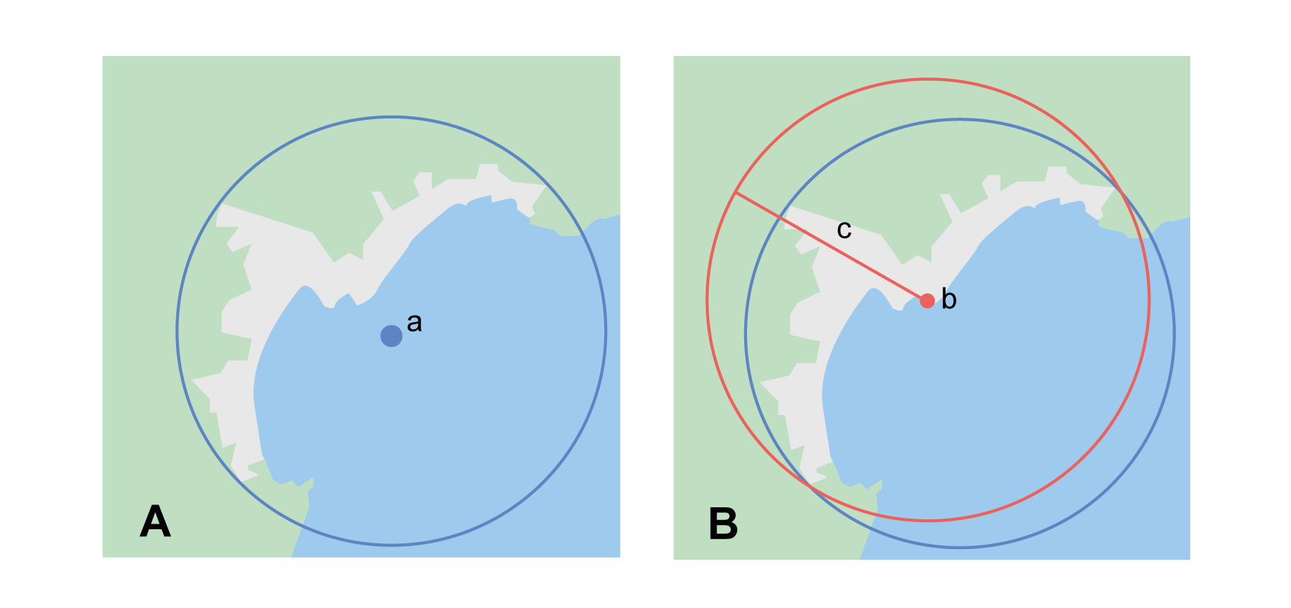
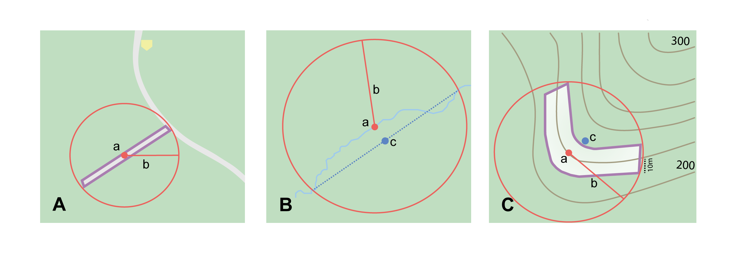
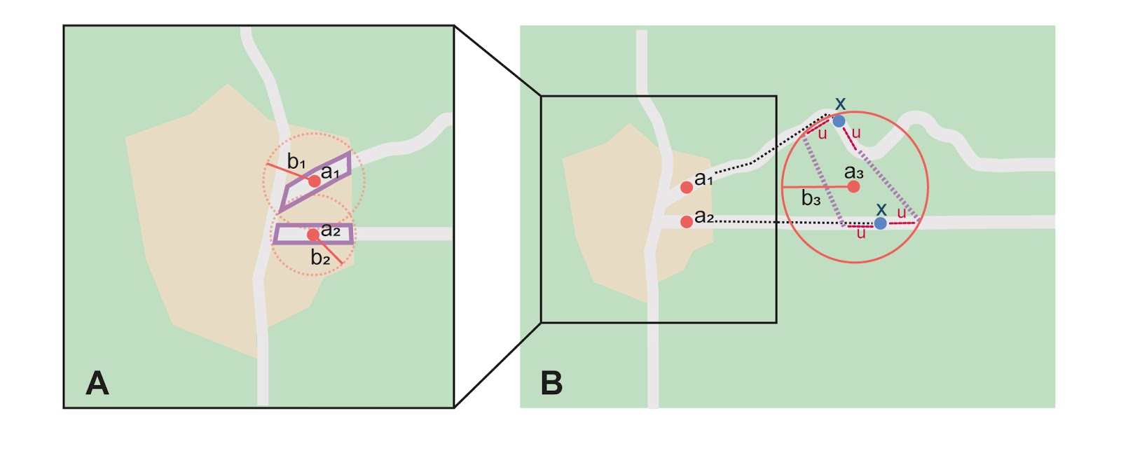
The corrected center is the point within a location, or on its boundary, that minimizes the geographic radial (see §1.6.3). This point is obtained by finding the smallest enclosing circle that contains the entire feature, and then taking the center of that circle (Figure 1A). If that center does not fall on or inside the boundaries of the feature, find the smallest enclosing circle that contains the entire feature, but has its center on the boundary of the feature (Figure 1B). Note that in the corrected case, the new circle, and hence the radial, will always be larger than the uncorrected one. In the Calculator, the coordinates corresponding to the corrected center are labelled as Input Latitude and Input Longitude. See Appendix B: Methods to Find the Corrected Center and Geographic Radial for techniques to determine the corrected center.
1.6.3. Radial of Feature
A feature is a place in the locality description that has an extent and can be delimited by a boundary. The geographic radial of the feature (shown as Radial of Feature in the Calculator) is the distance from the corrected center of the feature to the furthest point on the geographic boundary of that feature (see Figure 1 and Extent of a Location in Georeferencing Best Practices (Chapman & Wieczorek 2020)). Note that the radial was called "extent" in earlier documents and versions of the Calculator. See Appendix B: Methods to Find the Corrected Center and Geographic Radial for techniques to determine the geographic radial.
| The final georeference will have a geographic radial distinct from the geographic radial of any of the features in the locality description (because it will also encompass all sources of uncertainty), and once the calculation is performed, this will be displayed in the output from the Calculator in the Uncertainty field. |
1.6.4. Latitude
Labelled as Input Latitude in the Calculator. The geographic coordinate north or south of the equator (where latitude is 0) that represents the starting point for a georeference calculation and depends on the locality type.
Latitudes in decimal degrees north of the equator are positive by convention, while latitudes to the south are negative. The Calculator supports three degree-based geographic coordinate formats for latitude and longitude: decimal degrees (e.g. −41.0570673), degrees decimal minutes (e.g. 41° 3.424") and degrees minutes and seconds (e.g. 41° 3' 25.44" S).
1.6.5. Longitude
Labelled as Input Longitude in the Calculator. The geographic coordinate east or west of the prime meridian (an arc between the north and south poles where longitude is 0) that represents the starting point for a georeference calculation and depends on the locality type.
Longitudes in decimal degrees east of the prime meridian are positive by convention, while longitudes to the west are negative. The Calculator supports three degree-based geographic coordinate formats for latitude and longitude: decimal degrees (−71.5246934), degrees decimal minutes (71° 31.482") and degrees minutes and seconds (71° 31' 28.90" W).
1.6.6. Coordinate Source
The Coordinate Source is the type of resource (map type, GPS, gazetteer, locality description) from which the starting Input Latitude and Longitude were derived.
| More often than not, the original coordinates are used to find the general vicinity of the location on a map, after which the process of determining the corrected center provides the new coordinates. The Coordinate Source to use in the Calculator in this case is the map from which the corrected center was determined, not the original source used to determine the general vicinity on the map. For example, suppose the original coordinates came from a gazetteer, but the boundary and corrected center of the feature were determined from Google Maps, the Coordinate Source would be "Google Earth/Maps 2008", not "gazetteer". |
This term is related to, but NOT the same as, the Darwin Core term georeferenceSources, which requires the specific resources used rather than their type. Note that the uncertainties from the two sources gazetteer and locality description can not be anticipated universally, and therefore do not contribute to the global uncertainty in the calculations. If the error characteristics of these sources are known, they can be added in the Measurement Error field before calculating. If the source GPS is selected, the label for Measurement Error will change to GPS Accuracy, which is where the accuracy of the GPS (see Using a GPS in Georeferencing Best Practices (Chapman & Wieczorek 2020)) at the time the coordinates were taken should be entered.
1.6.7. Coordinate Format
The Coordinate Format in the Calculator defines the representation of the original geographic coordinates (decimal degrees, degrees minutes and seconds (DMS) or degrees decimal minutes) of the coordinate source.
| When the calculation type is not “Coordinates only”, the original coordinates are often used to find the general vicinity of the location on a map, after which the process of determining the corrected center provides the new coordinates. The Coordinate Format to use in the Calculator in this case is the coordinate format on the map from which the corrected center was determined, not the coordinate format of the original source used to determine the general vicinity on the map. For example, suppose the original coordinates came from a gazetteer in DMS, but the boundary and corrected center of the feature were determined from Google Maps, the Coordinate Format would be decimal degrees, not DMS. |
This term is only equivalent to the Darwin Core term verbatimCoordinateSystem if no conversions had to be performed from the original source to the format used in the Input Latitude and Input Longitude (e.g. if the original coordinates were UTM and you had to convert them to DMS, then the Coordinate Format in the Calculator will be DMS, but the verbatimCoordinateSystem will be UTM. Selecting the original coordinate format allows the coordinates to be entered in their native format and forces the Calculator to present appropriate options for coordinate precision. Changing the coordinate format will automatically reset the coordinate precision value to nearest degree. Be sure to correct this for the actual coordinate precision. The Calculator stores coordinates in decimal degrees to seven decimal places. This is to preserve the correct coordinates in all formats regardless of how many coordinate transformations are done.
1.6.8. Coordinate Precision
Labelled in the Calculator as Precision in the first column of input parameters, this drop-down list is populated with levels of precision in keeping with the coordinate format chosen. For example, with a Coordinate Format of degrees minutes seconds, an Input Latitude of 35° 22' 24" N and an Input Longitude of 105° 22' 28" W, the Coordinate Precision would be nearest second. A value of exact is any level of precision higher than the otherwise highest precision given on the list. Sources of coordinate precision may include paper or digital maps, digital imagery, GPS, gazetteers, or locality descriptions.
| The Coordinate Precision to use in the Calculator is the coordinate precision of the source from which the corrected center was determined, not the coordinate precision of the original source used to determine the general vicinity on the map. For example, suppose the original coordinates came from a gazetteer, but the boundary and corrected center of the feature were determined from Google Maps, the Coordinate Precision would be determined by the number of digits of decimal degrees you captured from the corrected center on Google Maps, not the Coordinate Precision of the coordinates from the original gazetteer entry. If you use all of the digits provided on Google Maps, the Coordinate Precision would be "exact". |
| This term is similar to, but NOT the same as, the Darwin Core term coordinatePrecision, which applies to the output coordinates. |
1.6.9. Datum
Defines the position of the origin and orientation of an ellipsoid upon which the coordinates are based for the given Input Latitude and Longitude (see coordinate reference system).
| The Datum to use in the Calculator is the datum (or ellipsoid) of the source from which the corrected center was determined. For example, suppose the original coordinates came from a gazetteer with an unknown datum, but the boundary and corrected center of the feature were determined from Google Maps, the Datum would be "WGS84", not "datum not recorded." |
The term Datum in the Calculator is equivalent to the Darwin Core term geodeticDatum. The Calculator includes ellipsoids on the Datum drop-down list, as sometimes that is all that coordinate source shows. The choice of datum in the Calculator has two important effects. The first is the contribution to uncertainty if the datum of the input coordinates is not known. If the datum and ellipsoid are not known, datum not recorded must be selected. Uncertainty due to an unknown datum can be severe and varies geographically in a complex way, with a worst-case contribution of 5359 m (see Coordinate Reference System in Georeferencing Best Practices (Chapman & Wieczorek 2020)). The second important effect of the datum selection is to provide the characteristics of the ellipsoid model of the earth, on which the distance calculations depend.
1.6.10. Direction
The Direction in the Georeferencing Calculator is the heading given in the locality description, either as a standard compass point (see Boxing the compass) or as a number of degrees in the clockwise direction from north. True North is not the same as Magnetic North (see Headings in Georeferencing Best Practices (Chapman & Wieczorek 2020)). If a heading is known to be a magnetic heading, it will have to be converted into a true heading (see NOAA’s Magnetic Field Calculator) before it can be used in the Calculator. If degrees from N is selected, a text box will appear to the right of the selection, into which the degree heading should be entered.
| Some marine locality descriptions reference a direction (azimuth) toward a landmark rather than a heading from the current location (e.g. "327° to Nubble Lighthouse"). To make a Distance a heading calculation for such a locality description, use the compass point 180 degrees from the one given in the locality description (147° in the example above) as the Direction. |
1.6.11. Offset Distance
The Offset Distance in the Calculator is the linear surface distance from a point of origin. Offsets are used for the Locality Types Distance at a heading and Distance only. If the Locality Type Distance along orthogonal directions is selected, there are two distinct offsets:
- North or South Offset Distance
-
The distance to the north or south (set with the selection box to the right of the distance text box) of the Input Latitude.
- East or West Offset Distance
-
The distance to the east or west (set with the selection box to the right of the distance text box) of the Input Longitude.
1.6.12. Distance Units
The Distance Units selection denotes the real world units used in the locality description. It is important to select the original units as given in the description. This is needed to incorporate the uncertainty from Distance Precision properly. If the locality description does not include distance units, use the distance units of the map from which measurements are derived.
-
select mi for "10 mi E (by air) Bakersfield"
-
select km for "3.2 km SE of Lisbon"
-
select km for measurements in Google Maps where the distance units are set to km.
1.6.13. Distance Precision
The Distance Precision, labelled in the Calculator as Precision in the second column of input parameters, refers to the precision with which a distance was described in a locality (see Uncertainty Related to Offset Precision in Georeferencing Best Practices (Chapman & Wieczorek 2020)). This drop-down list is populated based on the Distance Units chosen and contains powers of ten and simple fractions to indicate the precision demonstrated in the verbatim original offset.
-
select 1 mi for "6 mi NE of Davis"
-
select ¼ km for "3.75 km W of Hamilton"
1.6.14. Measurement Error
The Measurement Error accounts for error associated with the ability to distinguish one point from another using any measuring tool, such as rulers on paper maps or the measuring tools on Google Maps or Google Earth. The units of measurement must be the same as those in the locality description as captured in Distance Units (see §1.6.12). The Distance Converter at the bottom of the Calculator is provided to aid in changing a measurement to the locality description units. For example, a reasonable value for measurement error on a map is 1 mm, which on a map of 1:24,000 scale would be 24 m.
1.6.15. GPS Accuracy
When GPS is selected from the Coordinate Source drop-down list, the label for the Measurement Error text box changes to GPS Accuracy. We recommend entering a value that is at least twice the value given by the GPS at the time the coordinates were captured (see Uncertainty due to GPS in Georeferencing Best Practices (Chapman & Wieczorek 2020). If GPS Accuracy is not known, enter 100 m for standard hand-held GPS coordinates taken before 1 May 2000 when Selective Availability was discontinued. After that, use 30 m as a conservative default value.
1.6.16. Uncertainty
The Uncertainty in the Calculator is the calculated result of the combination of all sources of uncertainty (coordinate precision, unknown datum, data source, GPS accuracy, measurement error, feature extent, distance precision and heading precision) expressed as a linear distance – the geographic radial of the georeference and the radius in the point-radius method (Wieczorek et al. 2004). Along with the Output Latitude, Output Longitude, and Datum, the radius defines a circle containing all of the possible places a locality description could mean. In the Calculator the Uncertainty is given in meters.
2. Georeferencing Methods by Locality Type
2.1. Geographic Feature only
|
Definition
The simplest locality descriptions consist of only a named place, or more generally, a feature, which is often listed in a standard gazetteer and can probably be located on a map of the appropriate scale. |
Despite how they might be presented in a gazetteer or on a map, features are not points; they are areas that have a spatial extent. Some features can have an obvious spatial extent, while others may not. All variations of features are treated in this Guide as one or the other of these two main categories. The basic methodology is to try to determine the boundaries of the feature, its corrected center and a measure of how specific the feature is (defined here by the geographic radial). See Appendix B: Methods to Find the Corrected Center and Geographic Radial for techniques to determine the corrected center and geographic radial for various geometric types of features.
| Coordinates from geographic indexes such as gazetteers often use reference points that are not necessarily in the center of the feature. For example, a river may be referenced by its mouth, and a town by its main post office, courthouse, or main plaza. It is best to use a visual reference to determine boundaries, centers, and radials. For this reason, it is a good idea to use the gazetteer coordinates to find the feature on a map, and then use the map to find the boundaries, corrected center and geographic radial of the feature. |
2.1.1. Feature – with Obvious Spatial Extent
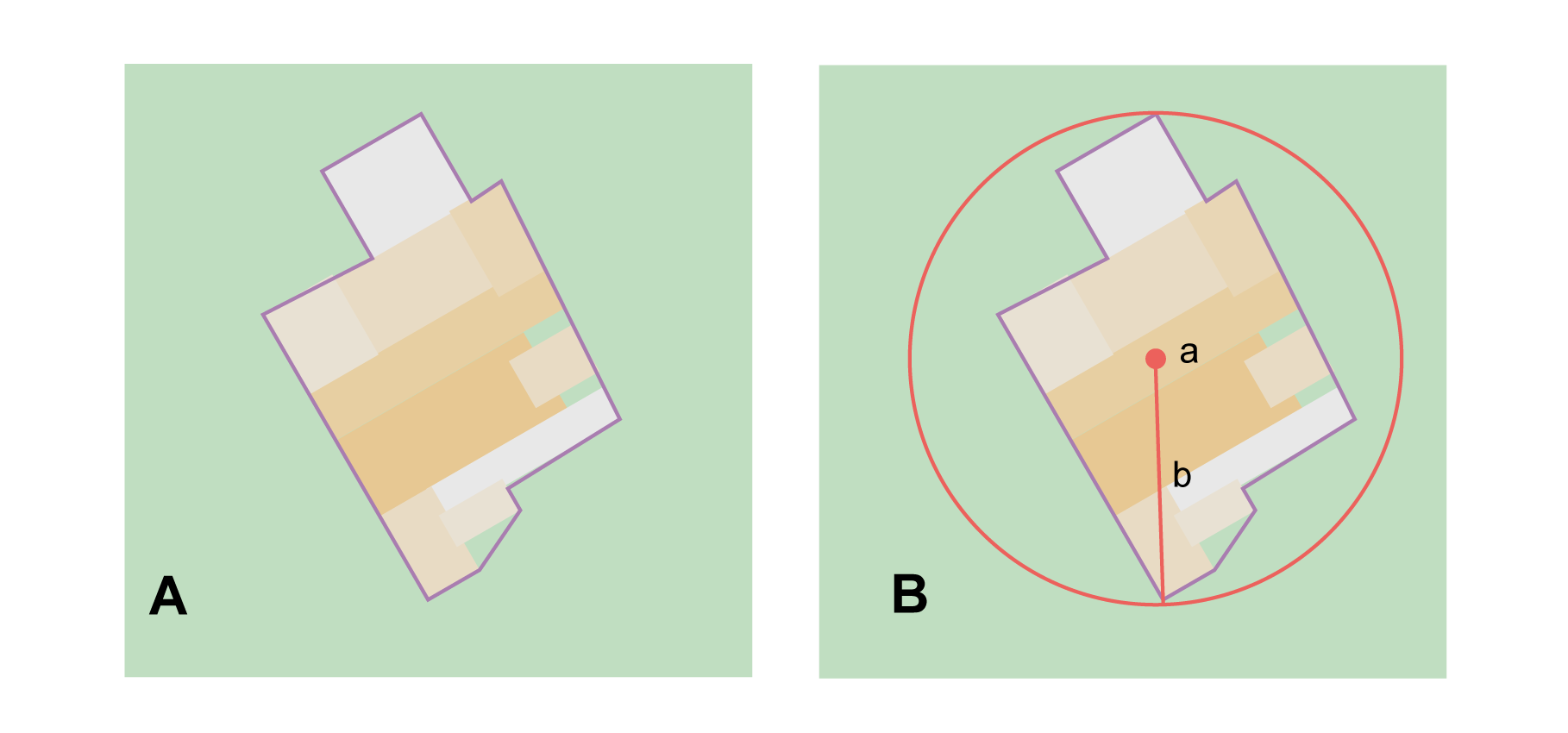
The locality refers to a geographic feature with discernible spatial extent, i.e. the boundaries of the feature can be determined easily (Figure 2).
-
"Puerto Madryn"
-
"Isla Tiburón"
-
"Yosemite National Park"
-
"Botany Bay"
Locality Type: Geographic feature only
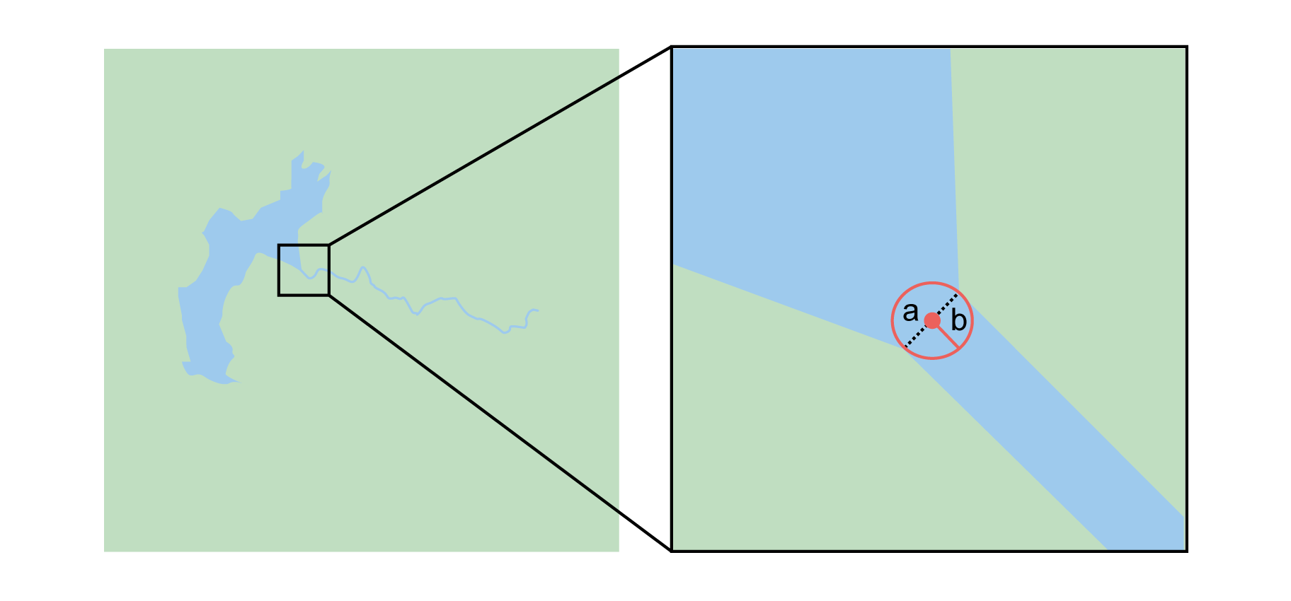
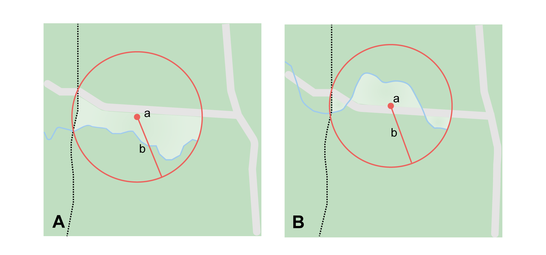
Step 1 – Determine the feature boundaries: This step is to determine the shape that contains the feature. This is typically done by drawing a polygon around the feature (Figure 2A), but some features may require more complex geometries, such as multiple polygons.
| Record the source (including date) used to determine the boundaries (see georeferenceSources). |
Step 2 – Determine the coordinates: Use the coordinates of the corrected center of the feature ("a" in Figure 2B) as the Input Latitude and Longitude.
Step 3 – Measure the geographic radial: Measure the distance from the corrected center to the furthest point on the boundary of the feature ("b" in Figure 2B) as the Radial of Feature.
Step 4 – Calculate using the following additional parameters in the Georeferencing Calculator: Coordinate Source, Coordinate Format, Datum, Coordinate Precision, GPS Accuracy/Measurement Error, and Distance Units (see §1.6).
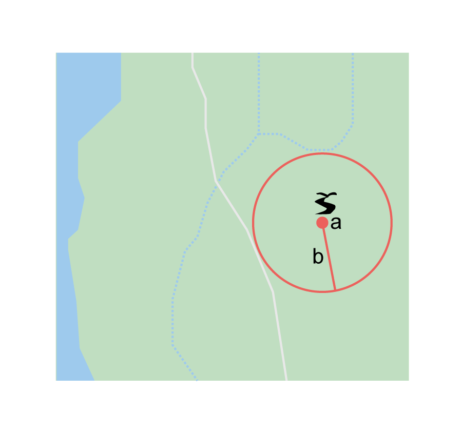
2.1.2. Feature – without Obvious Spatial Extent
The locality refers to a geographic feature that does not have an easily discernible spatial boundary. Some features may have undefined boundaries (e.g. mountains, unincorporated towns, etc.). Other features may only have a label, with no apparent boundaries or size on a map because they are small or obscured on satellite imagery (e.g. spring, monument, etc.). Another possibility is a feature with only coordinates from a gazetteer and no discernible presence on a map.
-
"Pampa Grande" as a region
-
"Mt Hypipamee"
-
"Great Barrier Reef"
Locality Type: Geographic feature only
Step 1 – Estimate the feature boundaries: Determine the boundaries of the feature as well as possible using visible evidence for the feature on a map. Try to get into the mind of the person who recorded the locality. Imagine yourself there. What circumstances would influence which feature was recorded and what circumstances would have encouraged them to choose a different feature?
For towns without obvious borders one can use the presence of buildings near the coordinates given for the town to decide where the town ends (Figure 3). In some cases there might not be such indicators and these will be more subjective. For this reason it is particularly important to document the rationale for the selection of the locality with unclear boundaries.
Where there are no indicators for the boundary, use the midpoint between the given feature and neighbouring features with similar type, size, or importance to make a rough boundary. Though this boundary may not represent the actual feature very well, it will represent the uncertainty of where the locality is, and that is the major goal of the georeference.
For small features, where the only indicator on a map is a label and possibly a marker, or where there are only coordinates from a gazetteer (and no further indicators at those coordinates on a map), a good strategy would be to use a predefined default size based on the feature type (Figure 4, Table 1).
Feature Type |
Default geographic radial |
|---|---|
spring, bore, tank, well, or waterhole |
3 m |
small stream |
3 m |
two-lane city streets, two-lane highways intersections |
10 m |
four-lane highways intersections |
20 m |
highway intersection, unknown type |
15 m |
PLSS Township |
6828 m |
PLSS Section |
1138 m |
PLSS ¼ Section |
570 m |
Grid (e.g. UTM), 1 m precision |
1 m |
Grid (e.g. UTM), 10 m precision |
7 m |
Grid (e.g. UTM), 100 m precision |
71 m |
Grid (e.g. UTM), 1 km precision |
707 m |
Grid, ¼ degree precision (at equator)† |
39226 m |
† Grids based on geographic coordinates, such as Quarter Degree Squares, are not square, nor are they constant. They vary in size and shape by latitude. See table in Uncertainty Related to Coordinate Precision in Georeferencing Best Practices (Chapman & Wieczorek 2020).
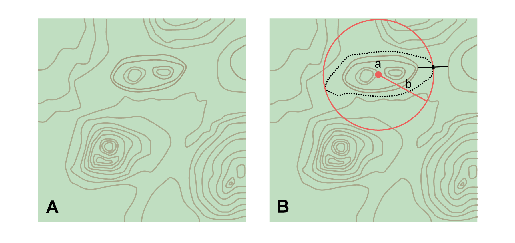
The boundaries between mountains can be determined by using the terrain (valleys, saddles, and plains) that separate one mountain from others around it (Figure 5).
Always use georeferenceRemarks to document the decisions made and the reasons for them as well as possible, including the neighbouring features used for reference.
Step 2 – Determine the coordinates: Once the estimated boundary has been determined, use the coordinates of the corrected center (Figure 2, Figure 3, and Figure 5B) as the Input Latitude and Longitude.
Step 3 – Measure the geographic radial: Once the rough boundary and the coordinates of the corrected center have been determined, find the geographic radial as the Radial of Feature by measuring the distance from the corrected center to the furthest point on the estimated boundary of the feature.
Step 4 – Calculate using the following additional parameters in the Georeferencing Calculator: Coordinate Source, Coordinate Format, Datum, Coordinate Precision, GPS Accuracy/Measurement Error, Distance Units (see §1.6).
2.1.3. Feature – Special Cases
The following are special cases of features that might or might not have an obvious spatial extent, depending on the completeness of the information available.
2.1.3.1. Feature – Street Address
The locality is a street address – usually with a number, a street name, and an administrative feature name.
-
"Av. Angel Gallardo 470, Buenos Aires, Argentina"
-
"1 Orchard Lane, Berkeley, CA"
-
"21054 Baldersleigh Road, Guyra, NSW" (indicates that the locality is 21.054 km from the beginning of Baldersleigh Road).
Locality Type: Geographic feature only
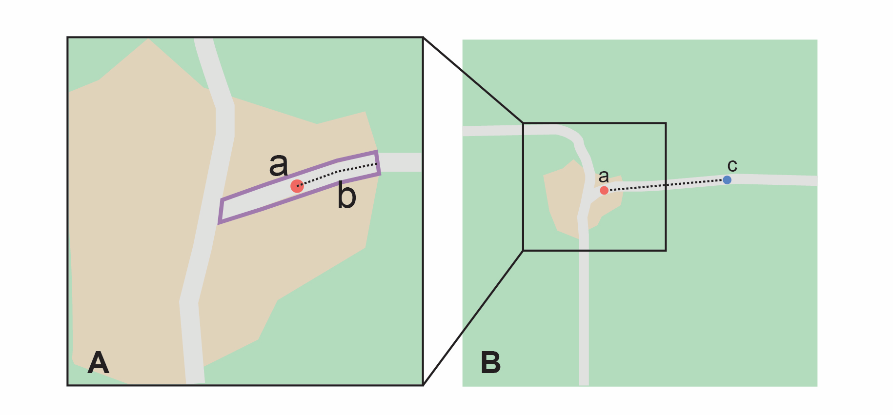
Step 1 – Determine the feature boundaries: Locate the address using a site such as Google Maps, Mapquest or OpenStreetMap.
-
Address boundary evident – if the map shows the extent of the address clearly, determine the boundary exactly as you would for a feature with an Obvious Spatial Extent (Figure 6A); (see §2.1.1).
-
Address boundary not evident – if the exact address cannot be found, estimate the boundary as well as possible, such as the block that it must be on (Figure 6B), as for §2.1.2. Many addresses reflect a grid system. For instance, addresses between 12th Street and 13th Street would lie between 1200 and 1300.
Step 2 – Determine the coordinates and geographic radial: Once the boundary has been determined, use the same method to determine the coordinates and geographic radial as for §2.1.1, namely, measure the distance from the coordinates of the corrected center to the furthest point on the boundary of the feature.
Step 3 – Calculate using the following additional parameters in the Georeferencing Calculator: Coordinate Source, Coordinate Format, Datum, Coordinate Precision, GPS Accuracy/Measurement Error, Distance Units (see §1.6).
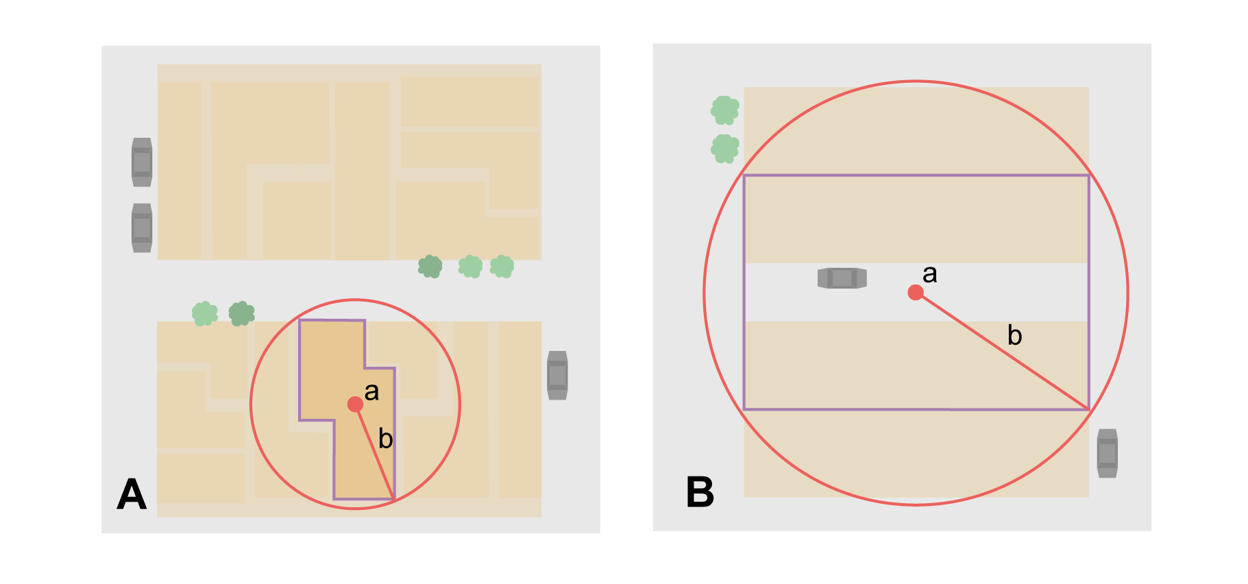
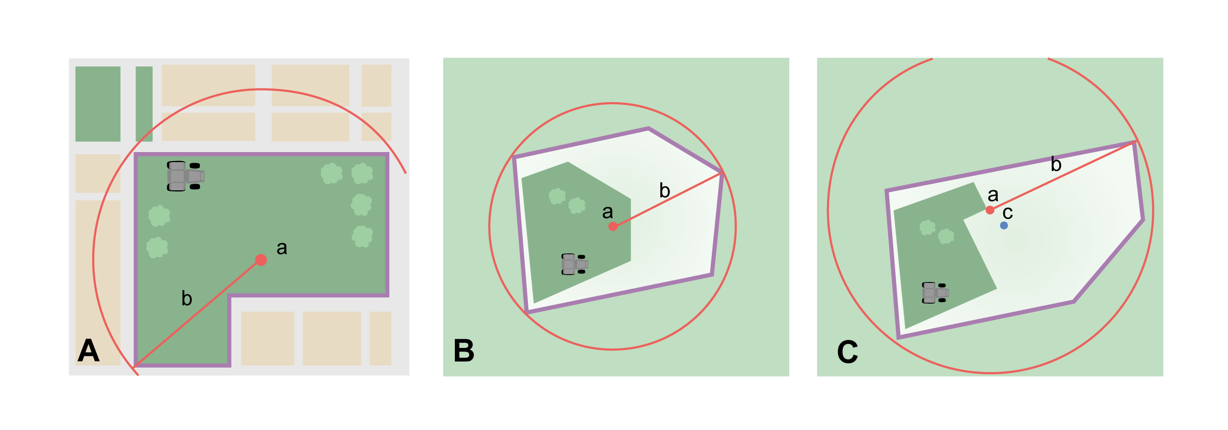
2.1.3.2. Feature – Property
The locality is a property – a ranch, rancho, station, farm, finca, grange, granja, estância, plantation, hacienda, fazenda, manor, holding, estate, spread, acreage, orchard, steading, parcel, terreno, etc.
-
"Victoria River Station"
-
"Mathae Ranch"
-
"Estancia 9 de Julio"
Locality Type: Geographic feature only
Step 1 – Determine the feature boundaries: Locate the property using whatever sources you can. You may have to resort to a cadastral map.
-
Property boundary evident – if the map shows the extent of the property, determine the boundary exactly as you would for §2.1.1).
-
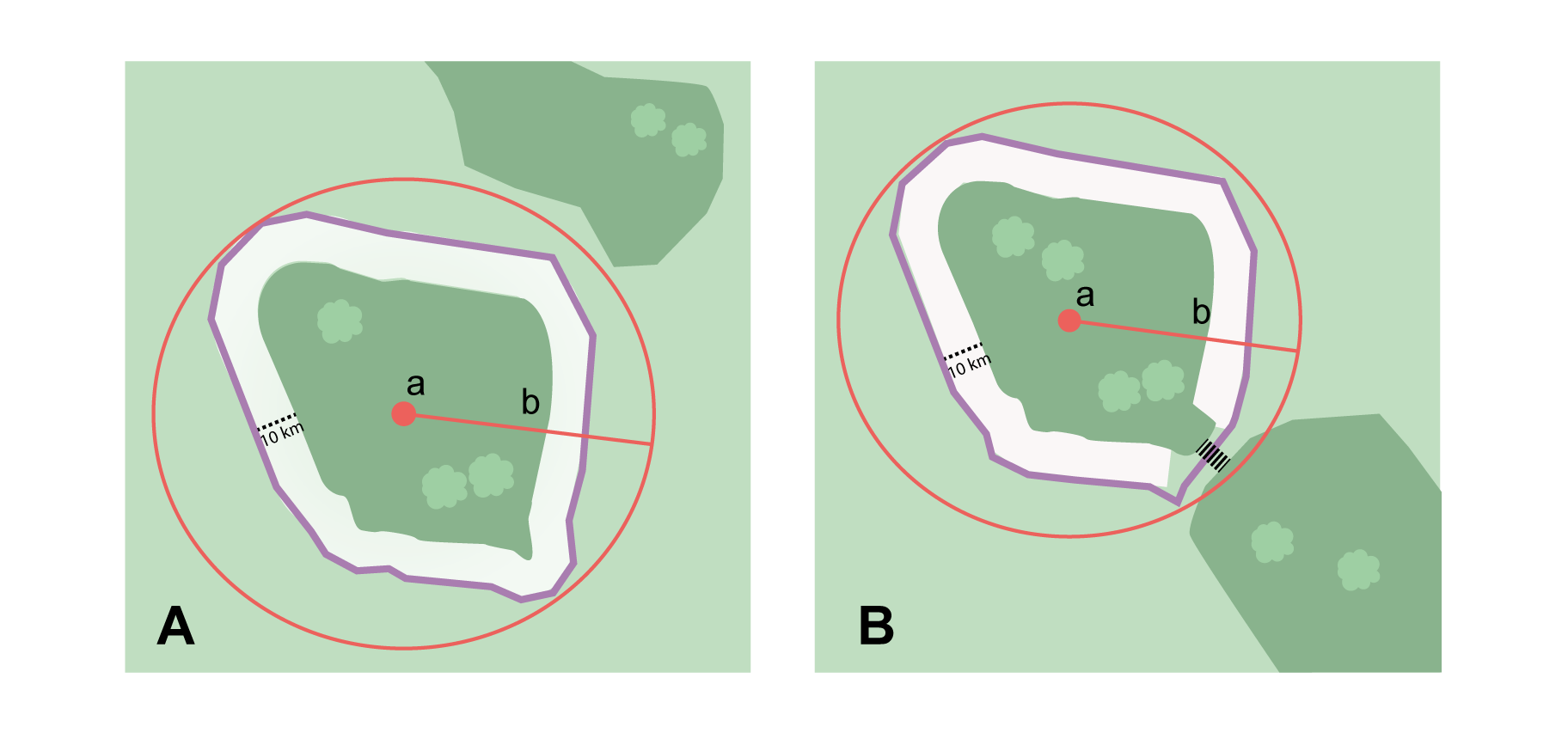
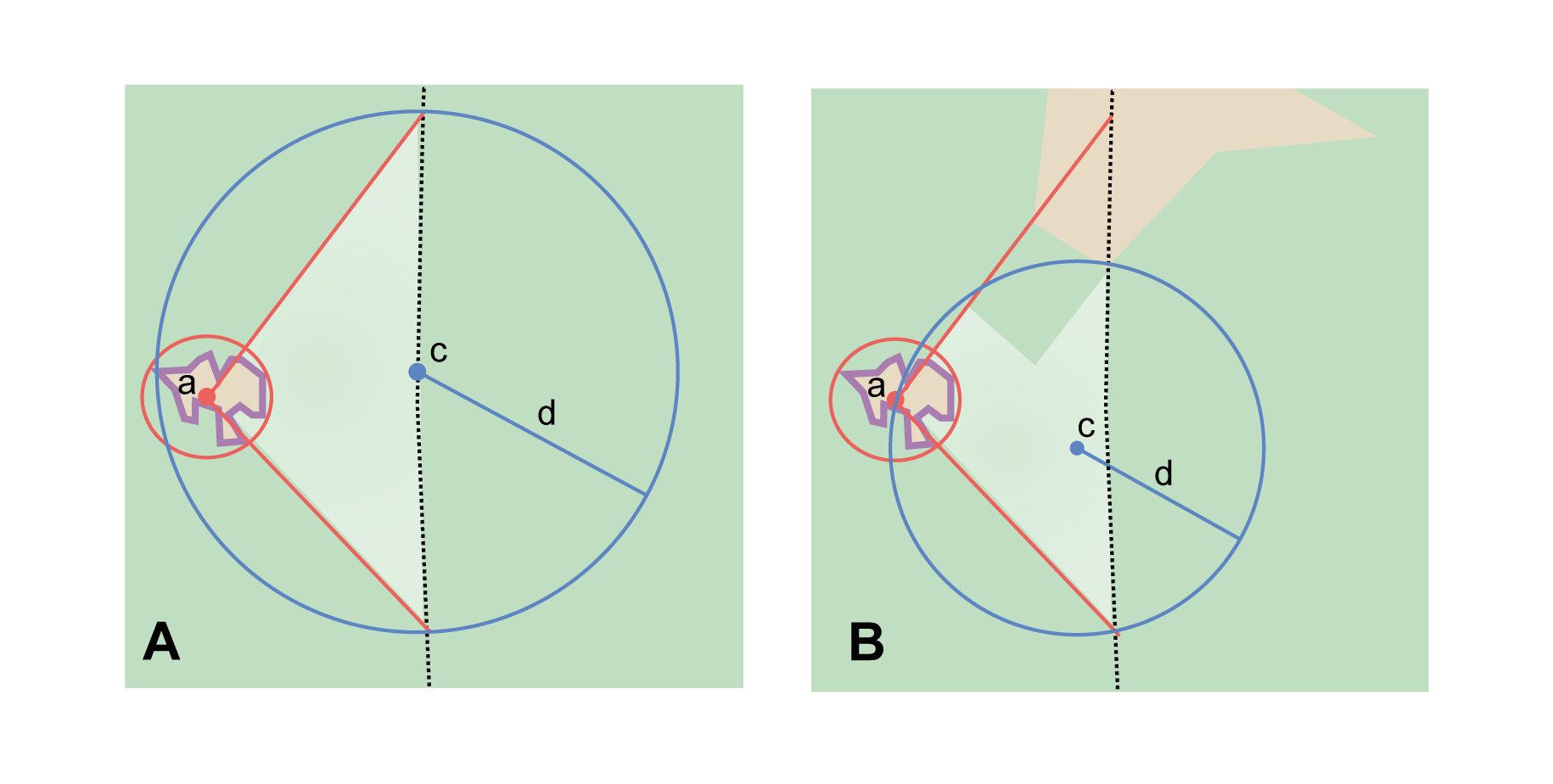
Property boundary not evident – if the full extent of the property cannot be found, it should still be possible to determine some part of it confidently, and the rest with less certainty. Delimit the outer, uncertain feature boundaries as usual by following §2.1.2. In addition, determine the boundaries of the part of the property that is obvious following §2.1.1.
Step 2 – Determine the coordinates and geographic radial:
-
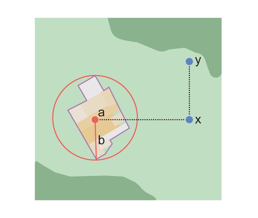
Property boundary evident – once the boundary is determined, determine the coordinates and geographic radial as for §2.1.1, namely, measure the distance from the coordinates of the corrected center to the furthest point on the boundary of the feature (Figure 7A).
-
Property boundary not evident – once the outer boundaries are determined, use them to find coordinates as for §2.1.1, namely find the center of the smallest enclosing circle containing the outer, uncertain boundary. If that center falls within the inner, confident boundary, use it to determine the geographic radial by finding the distance from that point to the furthest point on the uncertain boundary (Figure 7B). If the center does not fall in or on the confident inner boundary, let the corrected center be a point on the inner confident boundary that minimizes the geographic radial to the outer uncertain boundary (Figure 7C).
Step 3 – Calculate using the following additional parameters in the Georeferencing Calculator: Coordinate Source, Coordinate Format, Datum, Coordinate Precision, GPS Accuracy/Measurement Error, Distance Units (see §1.6).
2.1.3.3. Feature – Path
A path is a linear feature such as a road, trail, river, stream, contour line, boundary, transect, track of an animal’s movements, tow, trawl, etc. The locality may also refer to part (or subdivision) of a bigger path.
| A path may cross over itself, for example, as with the track of an animal’s movements. |
-
"Sacramento River"
-
"Arroyo Urugua-í"
-
"Hwy 1"
-
"along 100 m contour line"
Locality Type: Geographic feature only
Step 1 – Determine the feature boundaries: As a linear feature, a path is often represented as a series of line segments (i.e. a polyline), with or without a buffer. When viewed on satellite imagery these features (especially rivers) can be quite complex, so a constant buffer around the midline is not a good representation in these cases. When possible, determine the boundary as for any other shape using §2.1.1) (Figure 8A). Otherwise, treat the boundary as a polyline (Figure 8B) and determine the corrected center and geographic radial as explained below.
| Paths are susceptible to change over time, so it may be best to find a map source from the period during which the event occurred. The scale is important when looking at a path on a map, as smaller scale maps reduce the complexity shown, with corners cut off, and with loops (oxbows, billabongs), etc. often not shown. |
Contour Lines — these are linear features defined by elevation or depth. The horizontal width of the buffer around the contour line depends on the uncertainty in elevation or depth due to a combination of the stated range and the imprecision with which the value was recorded.
If a single value is given for an elevation (or depth knowing that the location was at the bottom of a waterbody), treat the path as a linear feature with a buffer around it, where the buffer is a vertical distance from the contour, not a horizontal one. The size of the vertical buffer should be equal to the precision with which the elevation is recorded. For example, if the precision is 100 feet (e.g. the precision of an elevation recorded as "2600 ft"), then the buffer is 100 vertical feet. Determine the shape of the feature using lines interpolated (or measured) one half of the buffer distance below the given contour and one half the buffer distance above the given contour (e.g. at 2550 feet and 2650 feet for the elevation example "2600 ft").
If an elevational range is given (e.g. 100-200 m), it is difficult to know whether the range was intended to encompass uncertainties in elevation or just the elevational bounds for the Location. To be conservative, we have to assume that it does not account for uncertainty in elevation and we need to add a buffer as described above around the upper and lower limits of the given range. For the example "100 - 200 m" the buffer is 100 m, so the lower boundary of the shape would be at 100 - 50 = 50 m and the upper boundary would be defined by 200 + 50 = 250 m.
| Buffers might require interpolation on a topographic map if they do not correspond with the printed contour lines (Figure 8C). |
These considerations can apply equally to bathymetry where contours are available, bearing in mind that some bathymetric contours are quite coarse and that most depths given in locality descriptions are actually above the bottom of the waterbody.
Step 2 – Determine the coordinates and geographic radial: If the boundary can be determined, treat as for §2.1.1, namely, measure the distance from the coordinates of the corrected center to the furthest point on the boundary of the feature (Figure 8A).
If the feature must be treated as a polyline, draw a straight line connecting the ends of the polyline and determine its midpoint. If the midpoint falls on the polyline, that will be the center (no need for correction), and the geographic radial will be the distance from that point to either of the endpoints of the polyline. If the midpoint does not fall on the polyline, move it to the point on the polyline that minimizes the distance to both endpoints. This is the corrected center and the distance to the endpoints is the geographic radial (Figure 8B).
Step 3 – Calculate using the following additional parameters in the Georeferencing Calculator: Coordinate Source, Coordinate Format, Datum, Coordinate Precision, GPS Accuracy/Measurement Error, Distance Units (see §1.6).
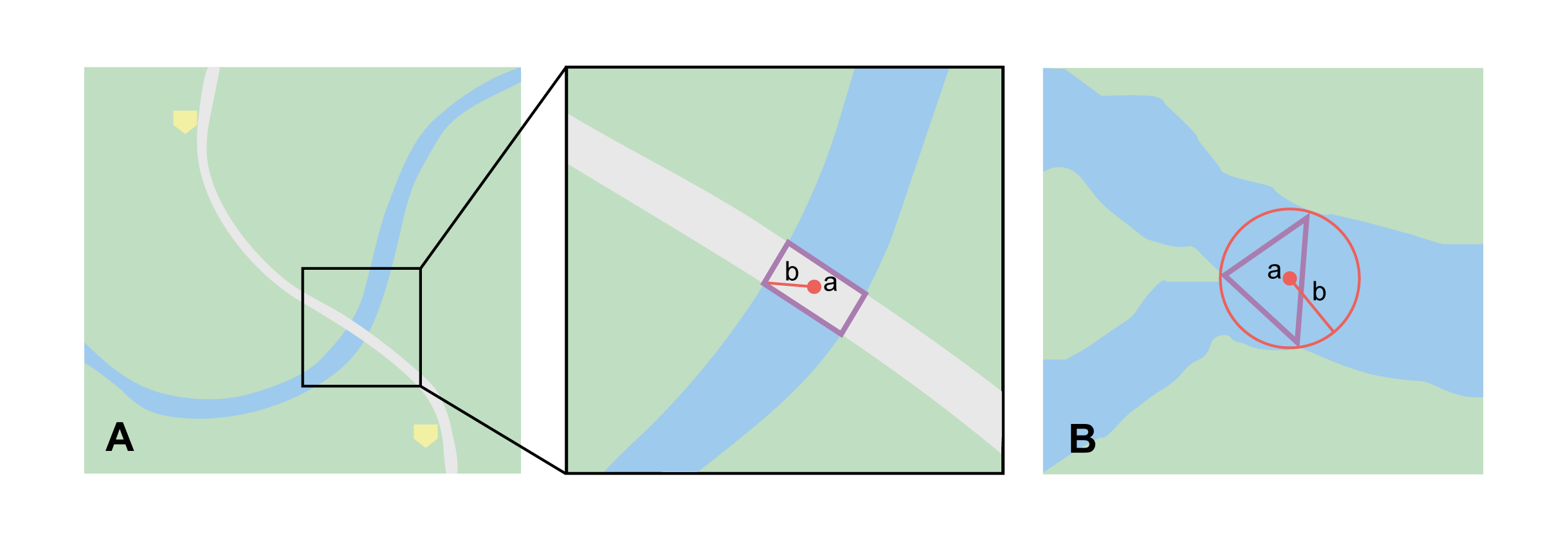
2.1.3.4. Feature – Junction, Intersection, Crossing, Confluence
The locality is the junction of two or more paths – roads, a road and a river, the mouth of a river (i.e. where it meets a larger water body), a road or river and an administrative boundary (e.g. of a park), a road and a contour line, etc.
-
"junction of Coora Rd. and E Siparia Rd"
-
"Where Dalby Road crosses Bunya Mountains National Park Boundary"
-
"confluence of Rio Claro and Rio La Hondura"
Locality Type: Geographic feature only
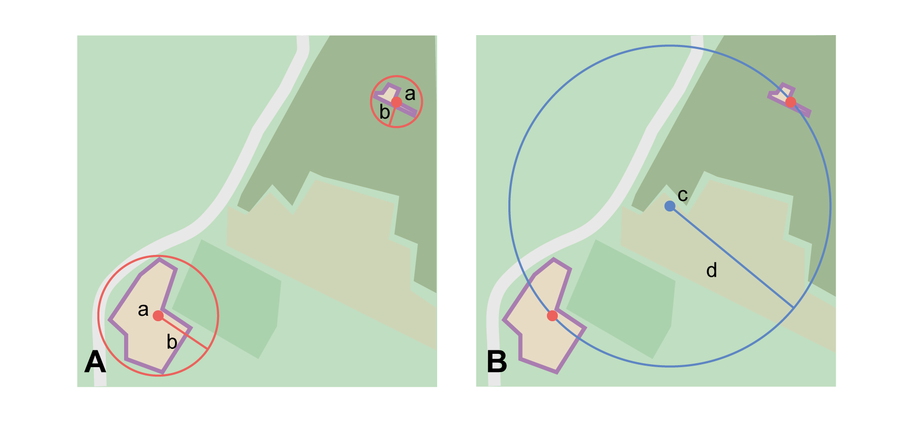
Step 1 – Determine the feature boundaries: Determine the boundary of the junction using routes of highways, roads, and rivers from resources such as Google Maps, Mapquest or OpenStreetMap, road atlases, GPS navigators, and satellite or aerial images (Figure 9A). Most modern spatial data can be used to determine the actual boundaries. If the only available representation of the junction shows the adjoining paths as lines, then the boundary must be determined as for §2.1.2.
For a confluence of two waterways, the boundary is a triangle that consists of the two segments at the same elevation reaching from where the waterways join to the opposite shores at the same elevation, plus the segment that joins those two points on the opposite shores (Figure 9B).
Step 2 – Determine the coordinates and geographic radial: Once the boundary has been determined, use the same method to determine the coordinates and geographic radial as for §2.1.1, namely, measure the distance from the coordinates of the corrected center to the furthest point on the boundary of the feature (Figure 9B).
Step 3 – Calculate using the following additional parameters in the Georeferencing Calculator: Coordinate Source, Coordinate Format, Datum, Coordinate Precision, GPS Accuracy/Measurement Error, Distance Units (see §1.6).
2.1.3.5. Feature – Cave
The locality is a cave, an underground mine, etc. For details of how to record a locality within a cave, see Caves in Georeferencing Best Practices (Chapman & Wieczorek 2020).
-
"Giant Dome, Hall of Giants, Carlsbad Caverns"
-
"Cueva de Las Brujas"
Locality Type: Geographic feature only
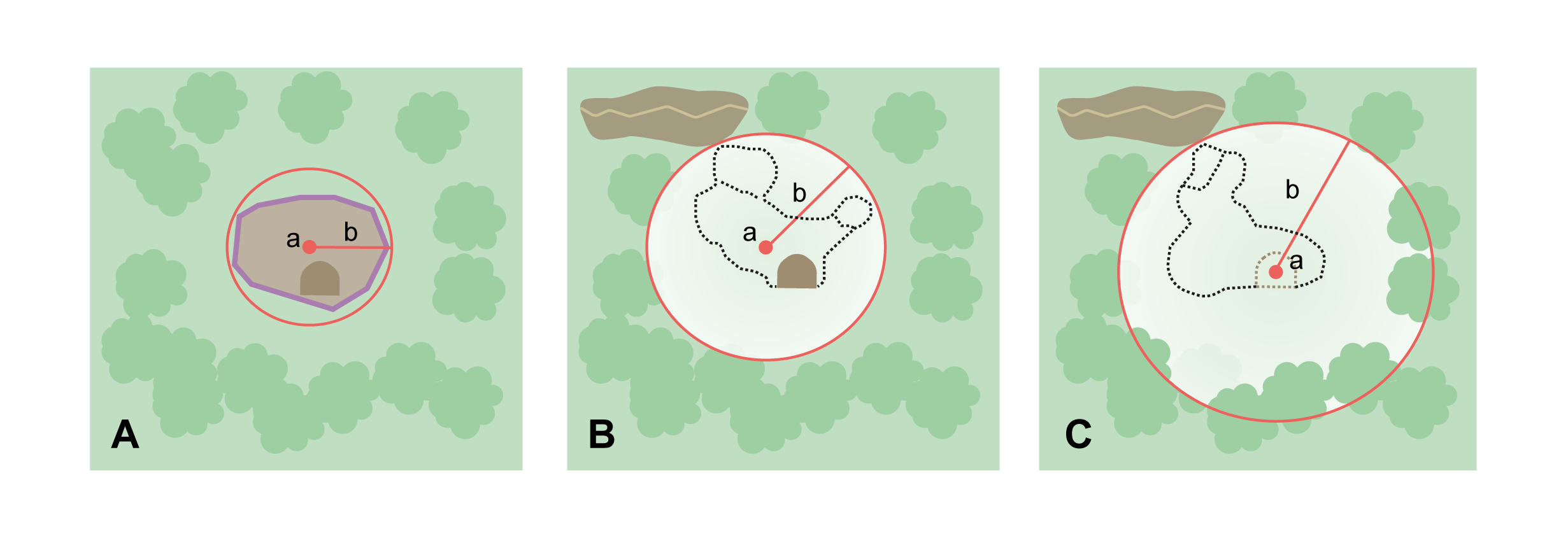
Step 1 – Determine the feature boundaries: Locate the cave and/or its main entrance.
-
Cave extent evident – if a map of all the interior of the cave with measurements and orientation to the surface is available, or if a position can be determined directly above the location inside the cave using the ground zero concept (see Determining Location in Georeferencing Best Practices (Chapman & Wieczorek 2020)), determine the boundary as if it is a §2.1.1 (Figure 10A).
-
Cave extent not evident – if the limits of the cave are not evident: a) use the nearest identifiable feature to determine the extent and boundary of the cave, as for §2.1.2 (Figure 10B); or b) determine the coordinates of the cave entrance and use any evidence of the size of the cave to circumscribe the boundary as a circle around the entrance with a radius commensurate with its size (Figure 10C). Document accordingly in georeferenceRemarks.
Step 2 – Determine the coordinates and geographic radial: Once the boundary has been determined, use the same method to determine the coordinates and geographic radial as for §2.1.1, namely, measure the distance from the coordinates of the corrected center to the furthest point on the boundary of the feature.
Step 3 – Calculate using the following additional parameters in the Georeferencing Calculator: Coordinate Source, Coordinate Format, Datum, Coordinate Precision, GPS Accuracy/Measurement Error, Distance Units (see §1.6).
2.1.3.6. Feature – Dive Location
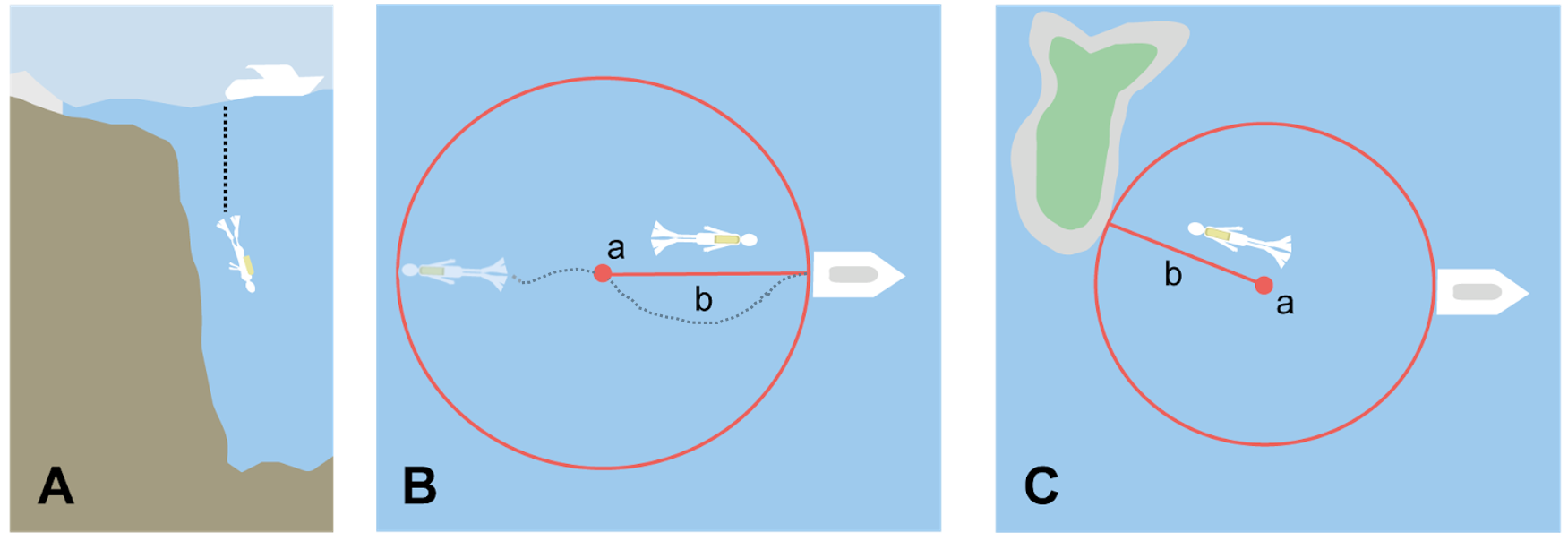
The locality is a marine or freshwater diving site. Commonly recorded using the geographic coordinates of the point on the surface where the diver entered the water (i.e. the entry point).
"Exploratory dive extending in a rough circle of 20 meters diameter between depths of 75 and 100 meters, beginning 100 meters south east of the entry point at a depth of 85 meters."
Locality Type: Geographic feature only
Step 1 – Determine the feature boundaries: Locate the extent of the dive as a 3D shape, which should be projected perpendicularly onto the water surface. Determine the boundary of that projection on the horizontal plane (i.e. the geographic boundary) (Figure 11).
-
Dive extent evident – underwater locations are often recorded as a distance, direction and water depth from the entry point. Below the surface there may be a "trajectory" with a three dimensional aspect that includes a horizontal component and a minimum and maximum water depth. Use these to circumscribe the boundary on the surface (see Figure 11A and Three Dimensional Shapes in Georeferencing Best Practices (Chapman & Wieczorek 2020)).
-
Dive extent not evident – if the limits of the dive are not evident, there is no trajectory, and no distance or direction from the entry point, use a reasonable upper limit for the distance the diver might have been able to cover in a straight line from and back to the entry point. This could vary greatly depending on the diver, the depth reached, equipment used, etc. Use any evidence of the length of the dive to circumscribe the boundary as a circle around the entry point with a radius commensurate with that length (Figure 11B).
Step 2 – Determine the coordinates and geographic radial: Treat as for §2.1.1, namely, measure the distance from the coordinates of the corrected center to the furthest point on the boundary of the feature.
Step 3 – Calculate using the following additional parameters in the Georeferencing Calculator: Coordinate Source, Coordinate Format, Datum, Coordinate Precision, GPS Accuracy/Measurement Error, Distance Units (see §1.6).
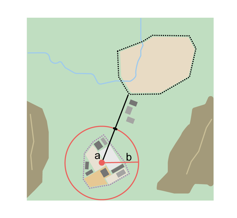
2.1.3.7. Feature – Headwaters of a Waterway
The headwater of a waterway may or may not be well defined. For most sizeable rivers a headwater is designated. If not, there is no universally agreed upon definition for a headwater. A reasonable interpretation might be the beginning of the most upstream first order stream that is a tributary of the named waterway. However, there is no guarantee that the author of the locality description used that definition. Therefore, we recommend the conservative solution that includes the watershed of all of the tributary streams of lower order than the waterway mentioned.
-
"headwaters of the Missouri River"
-
"Cabecera Río Manso"
Locality Type: Geographic feature only
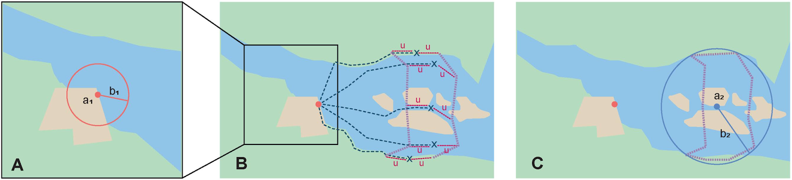
Step 1 – Determine the feature boundaries: Sometimes the position of a headwater is well known, e.g. it originates in a spring, lake, marsh, or a generally accepted beginning of a stream. If the headwater issues from a stationary waterbody such as a spring or lake, the feature is a line segment or polyline across the area where the water flows out of the stationary waterbody. In the latter case, treat the boundary as for a path (see §2.1.3.3), albeit a short one, as it is transverse to the flow of the waterway (Figure 12).
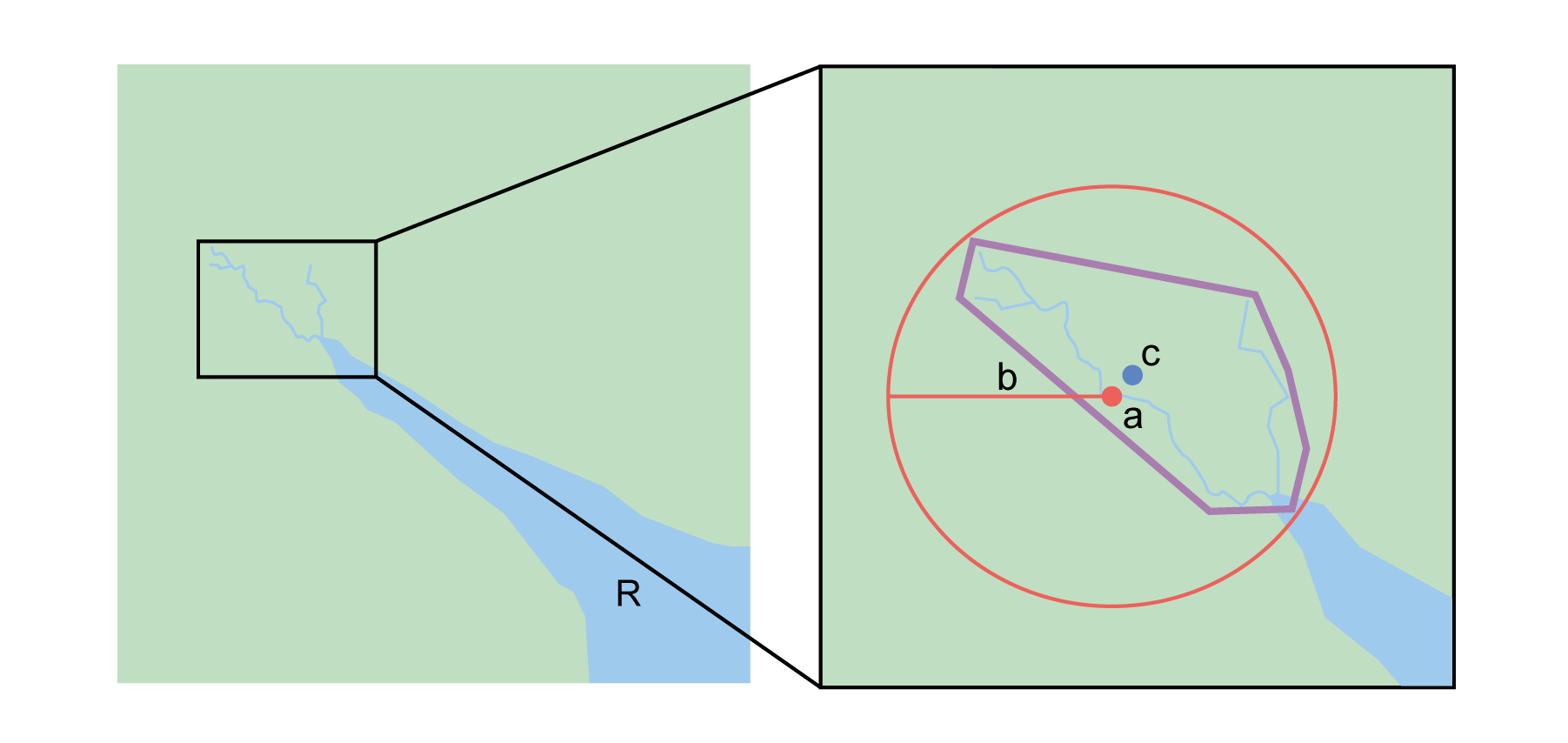
If the headwater is not designated, use the set of all of the streams upstream of the waterway mentioned. Draw the least convex polygon containing the entire set of streams as the boundary (Figure 13).
Step 2 – Determine the coordinates and geographic radial: Once the boundary has been determined, treat as for §2.1.1, namely, measure the distance from the coordinates of the corrected center to the furthest point on the boundary. The corrected center should be on a waterbody within the boundaries.
Step 3 – Calculate using the following additional parameters in the Georeferencing Calculator: Coordinate Source, Coordinate Format, Datum, Coordinate Precision, GPS Accuracy/Measurement Error, Distance Units (see §1.6).
2.1.3.8. Feature – near a Feature
The locality is given with a proximity to a feature, usually written as "near", "in the vicinity of", or "adjacent to", without any particular heading or distance. "Off" of a locality, often seen in marine locations, is included here, but in this case there is at least one constraint imposed by the shore.
-
"before Ceibas"
-
"near Dina Huapi"
-
"off Rottnest island"
-
"adjacent to the railway underpass on Smith Street"
Locality Type: Geographic feature only
Step 1 – Determine the feature boundaries: First determine the boundary of the feature that is mentioned in the description, based on the feature type, either as §2.1.1, or as §2.1.2. Then, to account for the proximity indicator, extend that boundary outward for a fixed distance in all directions (Figure 14A). Call this the "extended feature". If the extension overlaps the extension of any other similar feature, modify the boundary in the shared space to be half the distance between the nearest boundaries between the two features (Figure 14B).
| At the time the locality was recorded, neighbouring features might not have necessarily been in the same place as they are now. Also, features may have changed size in the time between the recording of the locality and the time when the map you use was made. These considerations add to the vagaries associated with this type of locality and underline the importance to never describe localities in this way. |
| The buffer distance for the extension is arbitrary – it is hard to defend any given value as a default. Make a judgement and imagine what the person who recorded the locality meant. Document the rationale and decisions made in dwc:georeferenceRemarks. |
Step 2 – Determine the coordinates and geographic radial: Once the boundary of the extended feature has been determined, treat as for §2.1.1, namely, measure the distance from the coordinates of the corrected center to the furthest point on the boundary of the extended feature.
Step 3 – Calculate using the following additional parameters in the Georeferencing Calculator: Coordinate Source, Coordinate Format, Datum, Coordinate Precision, GPS Accuracy/Measurement Error, Distance Units (see §1.6).
2.1.3.9. Feature – between Two Features
The locality description uses the pattern "between A and B", where A and B are two distinct features.
-
"between Missoula and Florence, Montana"
-
"Entre Pampa Blanca y Pampa Vieja, Jujuy"
-
"between Point Reyes and Inverness"
Locality Type: Geographic feature only
Step 1 – Determine the feature boundaries: Determine the boundaries of each feature as §2.1.1 or §2.1.2 (Figure 15A).
Step 2 – Determine the coordinates and geographic radial: Once you have determined the boundaries of the two features, find their corrected centers, as for §2.1.1. Use the midpoint between the corrected centers of the two features to determine the coordinates of the location between the features (Figure 15B). The geographic radial of the location between the two features is half the distance between the corrected centers of the features (Figure 15B).
Step 3 – Calculate using the following additional parameters in the Georeferencing Calculator: Coordinate Source, Coordinate Format, Datum, Coordinate Precision, Radial of Feature, GPS Accuracy/Measurement Error, Distance Units (see §1.6).
2.1.3.10. Feature – between Two Paths
The locality describes a location between two paths (two roads, two rivers, a road and a river, etc.).
-
"between the Great Western Hwy and the railway line"
-
"between Tanama R. and Clearwater Ck."
-
"entre Av. Corrientes y Av. Córdoba" (i.e. two streets that don’t intersect).
Locality Type: Geographic feature only
Step 1 – Determine the feature boundaries: Create a boundary that includes the two paths and any other boundaries that terminate those paths (e.g. the border of a given administrative division) (Figure 16A).
| Paths may cross each other one or more times, with the area between switching from one side of each path to the other, resulting in a boundary consisting of multiple polygons (Figure 16B). |
Step 2 – Determine the coordinates and geographic radial: Once the boundary has been determined, obtain the coordinates of the corrected center and the geographic radial as for §2.1.1, namely, measure the distance from the coordinates of the corrected center to the furthest point on the boundary of the feature.
Step 3 – Calculate using the following additional parameters in the Georeferencing Calculator: Coordinate Source, Coordinate Format, Datum, Coordinate Precision, GPS Accuracy/Measurement Error, Distance Units (see §1.6).
2.2. Offsets
|
Definition
An offset is a displacement from a reference location. An offset is usually used in conjunction with a heading to give a distance and direction from a feature (see Offsets and Uncertainty Related to Offset Precision in Georeferencing Best Practices (Chapman & Wieczorek 2020)). There are a variety of ways in which offsets with features and headings are represented in locality descriptions, each with its own methods of spatial interpretation. |
In all cases, both for the shape method and for the point-radius method using the Georeferencing Calculator, the boundaries of the reference feature(s) are needed. Thus, this section on Offsets will repeatedly refer to features as determined by the methods presented in the various sections of §2.1.
The locality types that involve offsets, in addition to the tricky one we have already seen above ("near a feature", §2.1.3.8), are:
-
distance only (e.g. "5 mi from Bakersfield")
-
heading only (e.g. "North of Bakersfield")
-
distance along a path (e.g. "13 miles east (by road) from Bakersfield")
-
distance along orthogonal directions (e.g. "2 miles east and 3 miles north of Bakersfield")
-
distance at a heading (e.g. "10 miles east (by air) from Bakersfield")
-
distances from two distinct paths (e.g. "1.5 miles east of Louisiana State Highway 1026 and 2 miles south of U.S. Highway 190")
2.2.1. Offset – Distance only
-
"5 km outside Calgary"
-
"12 km de Purmamarca"
Locality Type: Distance only
Step 1 – Determine the feature boundaries: Determine the boundary of the feature as you would for §2.1.3.8, except that the distance to use for the buffer is the distance given in the locality description, and there is no need to account for the proximity of other features.
Step 2 – Determine the coordinates and geographic radial: Once the boundary has been determined, obtain the coordinates and the geographic radial as for §2.1.1, namely, measure the distance from the coordinates of the corrected center to the furthest point on the boundary of the feature.
Offset Distance: Set to 0. The distance has already been incorporated in the determination of the boundary. Use the distance and units given in the locality description to georeference using the Georeferencing Calculator.
Distance Precision: Though the Offset Distance is set to zero, the Distance Precision should still be set (see §1.6.13) to account for this source of uncertainty.
Step 3 – Calculate using the following additional parameters in the Georeferencing Calculator: Coordinate source, Coordinate Format, Datum, Coordinate Precision, Measurement Error (see §1.6).
2.2.2. Offset – Heading only
The locality consists of a direction from a feature without any distance specified. Note that seldom is such information given alone; there is usually some supporting information. For example, the locality may have higher-level geographic information such as "East of Albuquerque, Bernalillo County, New Mexico". This provides a stopping point (the county border), and should allow you to georeference the locality. Alternatively, there might be another similar feature in the direction of the given heading that can constrain the offset.
-
"N Palmetto"
-
"W of Berkeley"
-
"Saladillo E"
-
"Al N de Saladillo"
Locality Type: Geographic feature only
Step 1 – Determine the feature boundaries: First determine the boundary of the given feature based on the feature type, either as for §2.1.1, or as for §2.1.2. Then, to account for the offset at a heading, extend that boundary outward in a cone defined by the heading uncertainty (see Offset – Direction Only and Uncertainty Related to Heading in Georeferencing Best Practices (Chapman & Wieczorek 2020)) until reaching a constraining boundary imposed by other information in the locality record, or until reaching the proximity of another similar feature, whichever is nearer to the original feature (Figure 17A). Call this the "extended feature". If the extension impinges on any similar extension of another similar feature in the cone of the specified heading, modify the boundary in the shared space to be half the distance between the nearest boundaries between the two features (Figure 17B). For example, "N Palmetto" could mean "northern part of Palmetto" or "North of Palmetto". Since we have no way of knowing which was intended, we choose the latter interpretation, which is more inclusive and will entirely contain the less inclusive interpretation. Use the rules for heading uncertainty to determine the angle within which to find the nearest similar feature. For example, for "N Palmetto" look for a named place somewhere between NE and NW of Palmetto.
Step 2 – Determine the coordinates and geographic radial: Once you have determined the boundary of the extended feature, treat as for §2.1.1, namely, measure the distance from the coordinates of the corrected center to the furthest point on the boundary of the extended feature.
Step 3 – Calculate using the following additional parameters in the Georeferencing Calculator: Coordinate Source, Coordinate Format, Datum, Coordinate Precision, GPS Accuracy/Measurement Error, Distance Units (see §1.6).
2.2.3. Offset – Distance along a Path
The locality consists of a reference feature to start from and a distance to travel along a path from there. Most of the time there will be just one path that matches the description and it will not be very wide compared to the reference feature, for example, a highway out of a town, or a stream out of a lake. In cases such as these, the georeferencing method is relatively simple (see §2.2.3.1). If the path is wide enough that multiple possible routes could be taken along it, such as in a wide river, the method for dealing with it is a little more complex (see §2.2.3.2). Sometimes there might be multiple distinct possible paths that match the locality description, such as two different roads in the same general matching direction out of a town, and there is a third method to use to find the georeference (see §2.2.3.3). In all cases, the georeference will cover a segment of the path or possible paths that includes all the sources of uncertainty. Though there might be a heading mentioned in the locality description (e.g. "9 km S El Bolsón on Ruta 40"), it serves only to constrain which path or paths are possible, and does not contribute uncertainty due to heading precision.
| The more accumulated curvature there is in the path, the more important it is to measure carefully (and therefore use a map of appropriate scale or zoom), otherwise there will be an accumulated error in the position of the offset. The less detail there is in the map compared to the real path, the greater the overestimate of the actual distance from the starting point to the end point will be because the measurements will be "cutting corners" along the whole measured path. |
| The more accumulated change in elevation there is along a path, the greater the deviation between the distance on the ground and the horizontal distance on a map. The distance on the ground is always greater than the corresponding horizontal distance. This effect is generally not very large, especially considering that localities of the type "Distance along a Path" follow a path that is traversable. Traversable roads and rivers can not have abrupt or excessive inclines. The only troublesome case is a walking path through steep terrain. No mainstream tools other than GIS, or measuring in situ again, permit the direct determination of distance on the ground. |
First let’s get an idea of how large the elevation effect can be, to understand the circumstances under which it is worth making the extra effort to estimate the distance on the ground. An important thing to understand is that the changes in elevation, both up and down, contribute to lengthen the route relative to the horizontal distance. The distance on the ground, on the path, is \$sqrt(x^2+y^2)\$, where \$x\$ is the projected horizontal distance and \$y\$ is the accumulated sum of changes in elevation. Note that the accumulated sum of changes in elevation is not necessarily the same as the final change in elevation between the starting point and the ending point of the trajectory. On a road, there could be ups and downs, and the sum of changes includes both, added as absolute values.
Let’s take an extreme case using the steepest road in the world, Baldwin Street in Dunedin, New Zealand. The street has a maximum grade of 35%. For comparison, highways with grades of 6% are usually considered steep enough to merit cautionary signage, and more than about 12% is rare to find. With a 35% grade, \$y\$ is 0.35 times \$x\$. Set \$x = 1\$ and do the calculation. The distance on the ground would be \$sqrt(0.35^2 + 1^2)\$ or 1.059 (5.9% longer). In a more normal extreme case of a 10% grade, the difference would be just 0.5%. Thus, under normal circumstances the difference is essentially negligible for roads and certainly so for navigable waters.
There are several ways to estimate distances on the ground without specialized tools or GIS. One way is to use an image of the elevation profile, which can be obtained using a screen capture in Google Earth Pro, for example. The image must be distorted so that the scale in both \$x\$ and \$y\$ is the same (1m elevation = 1m horizontal distance). With the image thus flattened, measure along the path of elevation and compare it to the length of the horizontal distance on the image.
A second way to estimate the distance on the ground is to sum all the elevation gains between pair-wise minima and maxima and do the same for all the pair-wise elevation losses. Sum the gains and losses (both as positive, because the rises and falls both contribute to positive length gains). Use that sum as the rise (\$y\$) in a slope calculation where the run (\$x\$) is the horizontal length of the path. From \$x\$ and \$y\$, calculate the distance on the ground as above.
A third way to estimate the distance on the ground is a gross simplification of the second method, above. Instead of measuring all pair-wise gains and losses, sum the net changes in elevation along three segments, 1) from the elevation at the beginning of the path to the lowest elevation, 2) the net change from the lowest elevation to the highest elevation, and 3) the net change from the highest elevation to the elevation at the end of the path.
2.2.3.1. Offset along a Narrow Path
-
"Ruta Nacional 81, 8 km O de Ingeniero Guillermo Nicasio Juárez"
-
"left bank of the Mississippi River, 16 mi downstream from St. Louis"
-
"500m up Skeleton Gorge"
Locality Type: Distance along path
Step 1 – Determine the starting feature boundaries: Find the boundary of the starting feature, which is the intersection of the reference feature with the path as you would for Feature – Junction, Intersection, Crossing, Confluence (Figure 18).
Step 2 – Determine the starting feature coordinates and length of the matching path: Once the boundary of the starting feature has been determined, find the midpoint along the path within the boundary of the feature it intersects with (Figure 18B). Note the distance along the path from the midpoint to the boundary of the feature it intersects in the direction of the offset. Enter the length of that segment in Radial of Feature in the Georeferencing Calculator.
Step 3 – Enter the Input Latitude and Longitude: Enter the coordinates of the offset position, which can be determined by measuring the length along the midline of the path from the midpoint found in the previous step to the distance along the path given in the locality description. See the notes on map scale and accumulated error in §2.2.3.
Step 4 – Calculate using the following additional parameters in the Georeferencing Calculator: Coordinate Source, Coordinate Format, Datum, Coordinate Precision, Measurement Error, Distance Units, Distance Precision (see §1.6).
2.2.3.2. Offset along a Wide Path
-
"Mississippi River, 16 mi downstream from St. Louis"
Locality Type: Distance along path
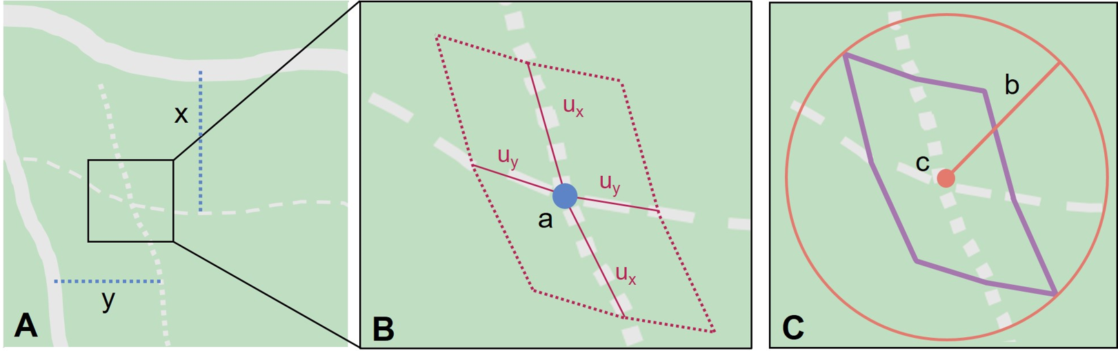
Step 1 – Determine the starting feature boundaries: Find the center of the starting feature, which is the intersection of the reference feature with the path as you would for Feature – Junction, Intersection, Crossing, Confluence (Figure 19A).
Step 2 – Determine the starting feature coordinates and geographic radial: Once the boundary of the starting feature has been determined, use the same method to determine the corrected center and geographic radial as for §2.1.1, namely, measure the distance from the coordinates of the corrected center to the furthest point on the boundary of the starting feature (Figure 19A).
Step 3 – Calculate preliminary uncertainties: Calculate a preliminary uncertainty by entering the geographic radial from Step 1 into the Radial of feature in the Georeferencing Calculator and fill in the rest of the parameters for the Distance along path locality type.
Additional parameters for Step 4: Coordinate Source, Coordinate Format, Datum, Coordinate Precision, Measurement Error, Distance Units, Distance Precision (see §1.6).
Step 4 – Final path boundary: The objective of this step is to estimate a boundary around the set of possible paths matching the description. To do so, we need to trace at least three of the possible paths. The first of these paths is from the coordinates of Step 2 along one side of the wide path to a distance equal to the offset distance given in the locality description. The second path is similar, but along the opposite side of the wide path starting at a point of equal elevation and tracing along that opposite side. The third path is from the coordinates of Step 2, along the middle of the wide path (or the deepest channel if locatable in the case of a waterway) to as far as to the offset distance given in the locality description. If there are other reasonably likely paths that are very different from these three, trace them in a similar manner. Each of these paths terminate at an X in the example in Figure 19B. From each of these termination points, trace both forward and backward to a distance equal to the uncertainty determined in Step 3 (the segments of the paths marked with u in Figure 19B). The outer endpoints of all the segments marked with u form a polygon (Figure 19B). This polygon is the final path boundary we seek.
Step 5 – Final corrected center and geographic radial: Once you have determined the boundary of the final boundary from Step 4, treat as for §2.1.1, namely, find the corrected center of the final path boundary and measure the distance from there to the furthest point on the boundary. Use the coordinates of the corrected center for the resulting Latitude and Longitude and use the length of the geographic radial of the final path boundary as the final Uncertainty. Use all of the rest of the output values from the calculation in Step 4 in the final georeference. No new calculation has to be made for this step.
2.2.3.3. Offset along Multiple Possible Paths
-
"15km al O de Rosario por ruta"
-
“5 km up Cox River from the coast, Limmen NP, NT, Australia” (Cox River is a delta with several arms).
Locality Type: As the locality type of the possible paths.
Step 1 – Determine the starting feature boundaries: Find the center of the intersection of the reference feature with each path as you would for Feature – Junction, Intersection, Crossing, Confluence (Figure 20A).
Step 2 – Determine the boundaries for distinct paths: For each of the distinct possible paths, determine the final boundaries of the path segment as for §2.2.3.1 or §2.2.3.2, as appropriate (Figure 20B).
Step 3 – Determine the final coordinates and geographic radial: Treat the set of boundaries from Step 2 and the minimum area between them as parts of the same feature. Find the corrected center and geographic radial for this combined feature (Figure 20B). Use the coordinates of the corrected center of this combined feature for the resulting Input Latitude and Longitude and use the length of the geographic radial of the combined feature as the final uncertainty. No further calculation is necessary.
2.2.4. Offset – Distance along Orthogonal Directions
The locality consists of a linear distance in each of two orthogonal directions from a feature. For more information and details see Offset along Orthogonal Directions in Georeferencing Best Practices (Chapman & Wieczorek 2020).
| Where localities have two orthogonal measurements in them, it should always be assumed that the measurements are "by air" unless there is a reference that indicates otherwise. |
-
"6 km N and 4 km W of Welna"
-
"2 mi E and 1.5 mi N of Kandy"
-
"2 miles north, 1 mile east of Boulder Falls, Boulder County, Colorado"
Locality Type: Distance along orthogonal directions
Step 1 – Determine the starting feature boundaries: Determine the boundary of the feature based on whatever the feature type is, either as for §2.1.1, or as for §2.1.2.
Step 2 – Determine the starting feature coordinates and geographic radial: Once the boundary of the starting feature has been determined, use the same method to determine the corrected center and geographic radial as for §2.1.1, namely, measure the distance from the coordinates of the corrected center to the furthest point on the boundary of the starting feature (Figure 21).
Step 3 – Calculate using the following additional parameters in the Georeferencing Calculator: Coordinate Source, Coordinate Format, Datum, Coordinate Precision, North or South Offset Distance, East or West Offset Distance, GPS Accuracy/Measurement Error, Distance Units, Distance Precision (see §1.6).
| For this type of calculation, the output coordinates are different from the Input Latitude and Input Longitude. |
2.2.5. Offset – Distance at a Heading
The locality consists of a distance in a given direction from a single feature. Such localities sometimes contain an explicit indicator of how the distance was measured, (e.g. "by air", "air miles W of", "due N of", "as the crow flies", "by road", "downstream from", etc.). Without such an indicator the interpretation is a matter of judgement, which should be documented in georeferenceRemarks.
| Since an offset at a heading "by air" will usually encompass the alternative by a path anyway, the former is the recommended locality type to use if there is no indication to the contrary. You can increase the maximum uncertainty to encompass the other option. This recommendation applies if you don’t have a compelling reason to use §2.2.3). |
| The addition of an adverbial modifier to the distance part of a locality description (e.g. "about 25 km WNW Campinas"), while an honest observation, should not affect the determination of the geographic coordinates or the overall uncertainty. |
-
"50 miles W of Las Vegas"
-
"10.2 km E de Amamá"
-
"16 mi downstream from St Louis on the Mississippi River"
-
"about 25 km WNW of Campinas"
-
"10 mi E (by air) Yerevan"
Locality Type: Distance at a heading
Step 1 – Determine the starting feature boundaries: Determine the boundary of the feature based on whatever the feature type is, either as for §2.1.1, or as for §2.1.2.
Step 2 – Determine the starting feature coordinates and geographic radial: Once the boundary has been determined, obtain the coordinates and the geographic radial as for §2.1.1, namely, measure the distance from the coordinates of the corrected center to the furthest point on the boundary of the feature.
Step 3 – Calculate using the following additional parameters in the Georeferencing Calculator: Coordinate Source, Coordinate Format, Datum, Coordinate Precision, Direction, Offset Distance, GPS Accuracy/Measurement Error, Distance Units, Distance Precision (see §1.6).
| For this type of calculation, the output coordinates are different from the Input Latitude and Input Longitude. |
2.2.6. Offset – Distances from Two Distinct Paths
-
"1.5 mi E LA Hwy. 1026 and 2 mi S U.S. 190"
Locality Type: Distance along path
Although this is not technically a distance along a path, the choice of this locality type in the Georeferencing Calculator will allow all of the relevant parameters to be entered.
Step 1 – Determine the feature boundaries: Determine the boundaries of the area matching the locality description by "transporting" each path by its given offset distance and direction. The transported paths will then overlap, each one having its corresponding buffer due to distance precision and path widths around it. This overlap of the two buffered areas defines the extent of the place described (Figure 22). Draw the boundary around the overlapping area.
Step 2 – Determine the coordinates and geographic radial: Once the boundary has been determined, obtain the coordinates and the geographic radial as for §2.1.1, namely, measure the distance from the coordinates of the corrected center to the furthest point on the boundary of the feature.
Step 3 – Calculate using the following additional parameters in the Georeferencing Calculator: Coordinate Source, Coordinate Format, Datum, Coordinate Precision, Radial of Feature, Measurement Error, Distance Units, Distance Precision (see §1.6).
2.3. Coordinates
|
Definition
The locality consists of a point represented by coordinates, which may be in the form of geographic coordinates (latitude and longitude), Universal Transverse Mercator (UTM), Quarter Degree Squares (QDS), metric grids, map sheets, or any number of other Cartesian reference systems |
2.3.1. Coordinates – Geographic Coordinates
The locality consists of a point represented by latitude and longitude coordinates in one of various coordinate formats:
-
degrees and decimal minutes (DDM)
-
decimal degrees (DD)
Records should also contain a hemisphere indicator ('E' or 'W' and 'N' or 'S' for DMS and DDM formats in English; '−' for west or south in DD format). For maritime locations, if there is no information that would suggest a particular Coordinate Source, use a map of 1:150000 scale, as this is a realistic conservative selection.
-
"36º 31' 21.4" N; 114º 09' 50.6" W" (DMS)
-
"36º 31.4566’N; 114º 09.8433’W" (DDM)
-
"−36.524276; −114.164055" (DD using minus signs to indicate southern and western hemispheres).
Locality Type: Coordinates only
Step 1 – Enter the coordinates: Enter the coordinates in the format they were captured from the GPS or from the verbatim locality (decimal degrees, degrees decimal minutes, or degrees minutes seconds) with all of the given digits of precision.
| The Georeferencing Calculator calculates and preserves seven digits of precision in decimal degrees so that any transformation between coordinate formats is reversible without introducing rounding errors. |
Step 2 – Calculate using the following additional parameters in the Georeferencing Calculator: Coordinate Source, Datum, Coordinate Precision, GPS Accuracy, Distance Units (see §1.6).
2.3.2. Coordinates – Universal Transverse Mercator (UTM)
The locality consists of a point represented by coordinate information in the form of Universal Transverse Mercator (UTM) or a related coordinate system. For UTM or equivalent coordinates, a Zone should ALWAYS be included to make sure that the longitude is not ambiguous. Zones are often not reported where a region (e.g. Tasmania) falls completely within one UTM zone. Be aware that UTM zones are valid only between 84°N and 80°S. For details on dealing with UTM Coordinates see Universal Transverse Mercator (UTM) Coordinates in Georeferencing Best Practices (Chapman & Wieczorek 2020).
| There are many national and local grids derived from UTM and that work in the same way, such as the Australian Map Grid (AMG). |
-
"N 4291492 E 456156"
-
"AMG Zone 56, x: 301545 y: 7011991"
-
"30T 699582 m east 5709431 m north"
Locality Type: Geographic feature only
Although this is not technically a feature, the Geographic feature only locality type in the Georeferencing Calculator includes all of the relevant parameters.
Step 1 – Convert the coordinates: The Universal Transverse Mercator UTM coordinates must be converted to decimal degrees using a UTM to Latitude/Longitude conversion tool. If the Zone is not given with the UTM coordinates, try to determine it using UTM Grid Zones of the World (Morton 2006) and any additional geographic information in the locality or geography fields combined with a UTM zone map. Use all of the digits of precision from the conversion in the Input Latitude and Longitude. Choose the Coordinate Source: Locality description
| UTM coordinates are sometimes truncated to fewer than 7 digits in the northing and 6 digits in the easting, signifying a less precise location. To make a coordinate conversion, add zeros to the right of each coordinate to make 7 digits overall in the northing and 6 digits in the easting. |
Step 2 – Determine geographic radial: If the UTM coordinates have 7 digits in the northing and 6 digits in the easting, the geographic radial is 0.707 m (because the coordinates distinguish to the nearest meter and the geographic radial is half the diagonal of the 1 m by 1 m grid cell). For UTM coordinates with fewer digits of precision see Table 1. This radial covers the uncertainty from the UTM coordinate precision. The Coordinate Precision in the Calculator for this case is the coordinate precision of the Input Latitude and Longitude, which depends on how many digits of decimal degrees are copied from the converted latitude and longitude (Table 1).
Step 3 – Calculate using the following additional parameters in the Georeferencing Calculator: Coordinate Format, Datum, Coordinate Precision, GPS Accuracy/Measurement Error, and Distance Units (see §1.6).
2.3.3. Coordinates – Grid Systems
Locality is a grid reference (see Grids in Georeferencing Best Practices (Chapman & Wieczorek 2020)), such as the 100 m square grids extensively used in Europe, Quarter Degree Square Grids (QDS) as used in South Africa, and the Public Land Survey System (PLSS) system of Townships andSection (TRS) used in the mid- and western USA. Townships in the PLSS system are usually square and six miles on each side, with 36 one-mile by one-mile sections. Be aware that not all townships are square, however, as some were adjusted to conform to administrative or natural boundaries (rivers, for example). Numbered Townships are not unique descriptions without a meridian, which often is not given in a locality description. The meridian must then be inferred from a Principal Meridian map using other information in the locality description. Similar subdivisions are used in other countries, and should be calculated in a similar way, once the sizes of the cells have been determined (see Table 1). Map sheets (quadrangles) are sometimes used and can also be calculated as a grid system. Note that, unlike geographic grids, QDS grids are referenced from the top left corner.
-
"E of Bakersfield, T29S R29E Sec. 34 NE ¼"
-
"QDS 3218CB"
-
"TQ2387" (Ordnance Survey National Grid)
Locality Type: Geographic feature only
Step 1 – Determine the coordinates: Determine as for §2.1.1. Use the coordinates for the corrected center of the named grid cell. Usually a grid is made up of bounding boxes, so determining the corrected center should be easy.
Step 2 – Determine the geographic radial: As for §2.1.1. See Table 1 for radials of regularly shaped Townships, Sections, and subsections.
Step 3 – Calculate using the following additional parameters in the Georeferencing Calculator: Coordinate Source, Coordinate Format, Datum, Coordinate Precision, Measurement Error, and Distance Units (see §1.6).
2.4. Difficult Localities
At times, locality descriptions are fraught with vagueness. This may be due to any number of reasons, but in particular relates to historic collections in areas that at may have had no named features to reference at the time when the locality was recorded. See the section Difficult Localities in Georeferencing Best Practices (Chapman & Wieczorek 2020).
A cause of vagueness may be incorrect data entry and it is recommended that checking the original catalogues, ledgers, field notes, specimen labels, etc. be the first step in removing the vagaries of a locality so that it can be georeferenced with confidence.
2.4.1. Dubious Locations
The most important type of vagueness in a locality description is one in which some or all of the locality is explicitly in question.
-
"possibly Isla Boca Brava"
-
"presumably central Chile"
-
"Bakersfield?"
Georeferencing procedure: If some part of the locality description is in question, but aside from that there is location information that is not in question, use the unquestioned part of the locality to determine the locality type and georeference it normally following the appropriate method. Document in georeferenceRemarks what had to be disregarded in order to georeference the locality in question. For example, for a locality “Argentina: Misiones, possibly Puerto Iguazú”, georeference “Misiones”, which is the most specific part of the locality that is not in question.
If the entire locality is in question, do not georeference it and document in georeferenceRemarks the reason for not georeferencing (e.g. "locality in question").
2.4.2. Cannot Be Located
The cited locality cannot be found, and there is no other location information in the record (e.g. no administrative divisions cited). This may be for any number of reasons, including:
-
There is no locality information cited.
-
The location fields contain other than location information.
-
The feature(s) cannot be found with available references.
-
"locality not recorded"
-
"Bob Jones"
-
"summit"
-
"200 m"
Do not georeference these localities. These recommendations apply to all locality types. Document in georeferenceRemarks the reason for not georeferencing, e.g. "locality cannot be found with available references". Fill in the georeferenceSources so that others do not waste time using the same resources to track down the locality.
2.4.3. More than One Matching Feature
At times the locality cannot be distinguished from among multiple possible candidates because the geographical feature in the locality description has multiple matches.
2.4.3.1. Multiple Related Nearby Features
-
"Nahuel Huapi" (could refer to a national park or a lake within it)
-
"Battle Mountain" (could refer to a mountain or a nearby town)
-
"San Isidro"
Locality Type: Geographic feature only
If there are multiple distinct nearby places with the same name and no further information to distinguish between the possibilities, such as "Battle Mountain" and the nearby town with the same name, treat the combination of them as the feature (Figure 23) and follow the procedure for the appropriate locality type. Make note of the multiple possibilities and the procedure used in georeferenceRemarks.
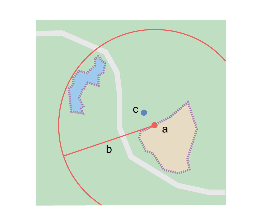
2.4.3.2. Multiple Unrelated Features
-
"Laguna Blanca" (could refer to distinct lagoons or municipalities in at least five different countries)
-
"Washington Street" (could refer to multiple streets in different places)
Do not georeference. Document in georeferenceRemarks the reason for not georeferencing, e.g. "there are multiple possible unrelated features matching the one in the locality description".
2.4.4. Demonstrably Inconsistent
The locality description contains irreconcilable inconsistencies – assertions that can not all be simultaneously true. Do not georeference these localities. Document in georeferenceRemarks the reason for not georeferencing, e.g. "locality contains irreconcilable inconsistencies".
A common source of inconsistency occurs when the locality description does not match the geopolitical subdivision of which it is supposed to be a part (e.g. "Missoula County, Idaho"). Elevation is another possible source of inconsistency, especially since elevation data are notoriously inaccurate (see Elevation in Georeferencing Best Practices (Chapman & Wieczorek 2020)). It is difficult to know which part of the locality is the one in error and a risk to judge that one part of the description should take precedence over another.
-
"Sonoma County side of the Gualala River, Mendocino County" (where the river runs between the counties mentioned)
-
"10 mi W of Bakersfield, 6000 ft" (There is no place anywhere near 10 mi W of Bakersfield at an elevation of 6000 ft)
-
"5 mi N of Delano, Kern Co." (5 mi N would put the locality in Tulare Co.)
Do not georeference. Rather than determine coordinates for such localities, annotate the locality in georeferenceRemarks with the nature of the inconsistency (e.g. "Missoula County not in Idaho") and refer the locality to the source institution for reconciliation.
2.4.5. Cultivated or Captive
The locality is recorded in association with a captive animal, a cultivated plant or some other non-natural occurrence. The locality cited is often that of a zoo, aquarium, botanical garden, etc. (see Dealing with Non-natural Occurrences in Georeferencing Best Practices (Chapman & Wieczorek 2020).
| The fact that an organism is recorded in a place out of its known or assumed natural distribution range does not constitute a problem from the point of view of locating that organism. Therefore, the determination of a georeference should not have any issues aside from those exclusively derived from the locality description itself (as seen for other cases above). This kind of information should instead be captured in the Darwin Core term degreeOfEstablishment. |
| If you are georeferencing based on location information only, and not together with the associated occurrence records, you may not have an easy way to capture other kinds of information (e.g. provenance, dates, degree of establishment, etc.). In these cases, it is recommended to amend the original occurrence records that contain the given locality to avoid any loss of information. |
-
"lab born, University of Oregon"
-
"bait shop"
-
"Cultivated in Botanic Gardens from seed obtained from Bourke, NSW."
-
"San Diego Wild Animal Park"
Georeference the locality normally based on the locality type and feature. Retain the location (e.g. zoo) along with its georeference, as for other localities in this Guide, but be sure to record the nature of its provenance (cultivated, captive, washed ashore, etc.) in the Darwin Core term degreeOfEstablishment.
Glossary
The purpose of this glossary is to describe important concepts in accordance with the intended meaning in this document, the associated Georeferencing Best Practices (Chapman & Wieczorek 2020) and the Georeferencing Calculator Manual (Bloom et al. 2020). These concepts are treated in broader contexts in many other sources. We have adapted the terms presented here from many sources including Wikipedia (as of November, 2019), the ESRI Dictionary (as of November, 2019) (ESRI n.d.), and various articles within Kemp 2008.
- accuracy
-
The closeness of an estimated value (for example, measured or computed) to a standard or accepted ("true") value. Antonym: inaccuracy Compare error, bias, precision, false precision and uncertainty.
"The true value is not known, but only estimated, the accuracy of the measured quantity is also unknown. Therefore, accuracy of coordinate information can only be estimated." (Geodetic Survey Division 1996, FGDC 1998). - bathymetry
-
-
The measure of depth of water in oceans, seas and lakes.
-
The shapes of underwater terrains, including underwater topography and sea floor mapping.
-
- boundary
-
The spatial divide between what is inside a location and what is outside of it.
- bounding box
-
An area defined by the coordinates of two diagonally opposite corners of a polygon, where those two corners define the north-south and east-west extremes of the area contained within.
- coordinate format
-
The format in which coordinates are encoded, such as "decimal degrees", "degrees minutes seconds", "degrees decimal minutes", or Universal Transverse Mercator UTM.
- coordinate precision
-
The fraction of a degree corresponding to the number of significant digits in the source coordinates. For example, if the coordinates are reported to the nearest minute, the precision is 1/3600th (0.00027778) of a degree; if a decimal degree is reported to two decimal places, the precision is 0.01 of a degree.
- coordinate reference system
-
(also spatial reference system) A coordinate system defined in relation to a standard reference or datum.
- coordinate system
-
A geometric system that defines the nature and relationship of the coordinates it uses to uniquely define positions. Examples include the geographic coordinate system and the Universal Transverse Mercator UTM coordinate system.
- coordinates
-
A set of values that define a position within a coordinate system. Coordinates are used to represent locations in space relative to other locations.
- corrected center
-
The point within a location, or on its boundary, that minimizes the geographic radial of the location. This point is obtained by making the smallest enclosing circle that contains the entire feature, and then taking the center of that circle. If that center does not fall inside the boundaries of the feature, make the smallest enclosing circle that has its center on the boundary of the feature. Note that in the second case, the new circle, and hence the radial, will always be larger than the uncorrected one (see Figure 1).
- Darwin Core
-
A standard for exchanging information about biological diversity (see Darwin Core).
- datum
-
A set of one or more parameters that serve as a reference or basis for the calculation of other parameters ISO 19111. A datum defines the position of the origin, the scale, and the orientation of the axes of a coordinate system. For georeferencing purposes, a datum may be a geodetic datum or a vertical datum.
- decimal degrees
-
Degrees expressed as a single real number (e.g. −22.343456). Note that latitudes south of the equator are negative, as are longitudes west of the prime meridian to −180 degrees. See also decimal latitude and decimal longitude.
- depth
-
A measurement of the vertical distance below a vertical datum. In this document, we try to modify the term to signify the medium in which the measurement is made. Thus, "water depth" is the vertical distance below an air-water interface in a waterbody (ocean, lake, river, sinkhole, etc.). Compare distance above surface. Depth is always a non-negative number.
- direction
-
see heading.
- DMS
-
Degrees, minutes and seconds – one of the most common formats for expressing geographic coordinates on maps. A degree is divided into 60 minutes of arc and each minute is divided into 60 seconds of arc. Degrees, minutes and seconds are denoted by the symbols °, ′, ″. Degrees of latitude are integers between 0 and 90, and should be followed by an indicator for the hemisphere (e.g. N or S). Degrees of longitude are integers between 0 and 180, and should be followed by an indicator for the hemisphere (e.g. E or W).
- easting
-
Within a coordinate reference system (e.g. as provided by a GPS or a map grid reference system), the line representing eastward distance from a reference meridian on a map.
- elevation
-
A measurement of the vertical distance of a land or water surface above a vertical datum. On maps, the reference datum is generally some interpretation of mean sea level or the geoid, while in devices using GPS/GNSS, the reference datum is the ellipsoid of the geodetic datum to which the GPS unit is configured, though the device may make corrections to report the elevation above mean sea level or the geoid. Elevations that are above a reference point should be expressed as positive numbers, while those below should be negative. Compare depth, distance above surface, and altitude.
- ellipsoid
-
A three-dimensional, closed geometric shape, all planar sections of which are ellipses or circles. An ellipsoid has three independent axes. If an ellipsoid is made by rotating an ellipse about one of its axes, then two axes of the ellipsoid are the same, and it is called an ellipsoid of revolution. When used to represent a model of the earth, the ellipsoid is an oblate ellipsoid of revolution made by rotating an ellipse about its minor axis.
- entry point
-
The entry point on the surface of the ocean or lake where a diver enters the water and from which all activities are measured. See illustration in Georeferencing Best Practices (Chapman & Wieczorek 2020).
- error
-
The difference between a computed, estimated, or measured value and the accepted true, specified, or theoretically correct value. It encompasses both the imprecision of a measurement and its inaccuracies. Error can be either random or systematic. If the error is systematic, it is called "bias". Compare accuracy, bias, precision, false precision and uncertainty.
- extent
-
The entire space within the boundary a location actually represents. The extent can be a volume, an area, or a distance.
- feature
-
An object of observation, measurement, or reference that can be represented spatially. Often categorized into "feature types" (e.g. mountain, road, populated place, etc.) and given names for specific instances (e.g. "Mount Everest", "Ruta 40", "Istanbul"), which are also sometimes referred to as "named places", "place names" or "toponyms".
- gazetteer
-
An index of geographical features and their locations, often with geographic coordinates.
- geocode
-
The process (verb) or product (noun) of determining the coordinates for a street address. It is also sometimes used as a synonym for georeference.
- geographic boundary
-
The representation in geographic coordinates of a vertical projection of a boundary onto a model of the surface of the Earth.
- geographic center
-
The midpoint of the extremes of latitude and longitude of a feature. Geographic centers are relatively easy to determine, but they generally do not correspond to the center obtained by a least circumscribing circle. For that reason it is not recommended to use a geographic center for any application in georeferencing. Compare corrected center.
- geographic coordinates
-
A measurement of a location on the Earth’s surface expressed as latitude and longitude.
- geographic radial
-
The distance from the corrected center of a location to the furthest point on the geographic boundary of that location. The geographical radial is what contributes to calculations of the maximum uncertainty distance using the point-radius georeferencing method. The term geographic radial, as defined here, replaces its equivalent "extent" used in the early versions of this Quick Reference Guide and related documents.
- geometry
-
The measures and properties of points, lines, and surfaces. Geometry is used to represent the geographic component of locations.
- georeference
-
The process (verb) or product (noun) of interpreting a locality description into a spatially mappable representation using a georeferencing method. Compare with geocode. The usage here is distinct from the concept of georeferencing satellite and other imagery (known as georectification).
- georeferencing method
-
The theory, including a set of rules, general procedures and expected outcomes, meant to produce a specific type of spatial representation of a locality.
- georeferencing protocol
-
The set of specific documented steps that can be applied to produce a spatial representation of a locality, following one or more georeferencing methods.
- GPS
-
Global Positioning System, a satellite-based system used for determining positions on or near the Earth. Orbiting satellites transmit radio signals that allow a receiver to calculate its own location as coordinates and elevation, sometimes with accuracy estimates. See also GNSS of which GPS is one example. See also GPS (receiver).
- GPS (receiver)
-
The colloquial term used to refer to both GPS and GNSS receivers (including those in smartphones and cameras). A GPS or GNSS receiver is an instrument which, in combination with an inbuilt or separate antenna, is able to receive and interpret radio signals from GNSS satellites and translate them into geographic coordinates.
- grid
-
A network or array of evenly spaced orthogonal lines used to organize space into partitions. Often these are superimposed on a map and used for reference, such as Universal Transverse Mercator UTM grid.
- ground zero
-
The location on the land surface directly above a radiolocation point in a cave where the magnetic radiation lines are vertical. See illustration in Georeferencing Best Practices (Chapman & Wieczorek 2020).
- heading
-
Compass direction such as east or northwest, or sometimes given as degrees clockwise from north. Usually used in conjunction with offset to give a distance and direction from a feature.
- latitude
-
The angular distance of a point north or south of the equator.
- locality
-
The verbal representation of a location, also sometimes called locality description.
- locality clause
-
A part of a locality description that can be categorized into one of the locality types, to which a specific georeferencing protocol can be applied.
- locality type
-
A category applied to a locality clause that determines the specific georeferencing protocol that should be used.
- location
-
A physical space that can be positioned and oriented relative to a reference point, and potentially described in a natural language locality description. In georeferencing, a location can have distinct representations based on distinct rules of interpretation, each of which is embodied in a georeferencing method.
- longitude
-
The angular distance of a point east or west of a prime meridian at a given latitude.
- meridian
-
A line on the surface of the Earth where all of the locations have the same longitude. Compare antimeridian and prime meridian.
- northing
-
Within a coordinate reference system (e.g. as provided by a GPS or a map grid reference system), the line representing northward distance from a reference latitude.
- offset
-
A displacement from a reference location. Usually used in conjunction with heading to give a distance and direction from a feature.
- path
-
A route or track between one place and another. In some cases the path may cross itself.
- point-radius
-
A representation of the geographic component of a location as geographic coordinates and a maximum uncertainty distance. The point-radius georeferencing method produces georeferences that include geographic coordinates, a coordinate reference system, and a maximum uncertainty distance that encompasses all of the possible geographic coordinates where a locality might be interpreted to be. This representation encompasses all of the geographical uncertainties within a circle. The point-radius method uses ranges to represent the non-geographic descriptors of the location (elevation, depth, distance above surface).
- precision
-
-
The closeness of a repeated set of observations of the same quantity to one another – a measure of control over random error.
-
With values, it describes the finest unit of measurement used to express that value (e.g. if a record is reported to the nearest second, the precision is 1/3600th of a degree; if a decimal degree is reported to two decimal places, the precision is 0.01 of a degree).
Antonym: imprecision. Compare accuracy, error, bias, false precision, and uncertainty.
-
- prime meridian
-
The set of locations with longitude designated as 0 degrees east and west, to which all other longitudes are referenced. The Greenwich meridian is internationally recognized as the prime meridian for many popular and official purposes.
- radial
-
The distance from a center point (e.g. the corrected or geographic center) within a location to the furthest point on the outermost boundary of that location. See also geographic radial.
- shape
-
synonym of footprint. A representation of the geographic component of a location as a geometry. The result of a shape georeferencing method includes a shape as the geographic component of the georeference, which contains the set of all possible geographic coordinates where a location might be interpreted to be. This representation encompasses all of the geographical uncertainties within the geometry given. The shape method uses ranges to represent the non-geographic descriptors of the location (elevation, depth, distance above surface).
- smallest enclosing circle
-
A circle with the smallest radius (radial) that contains all of a given set of points (or a given shape) on a surface (see Smallest-circle problem). This is seldom the same as the geographic center, nor the midpoint between two most distant geographic coordinates of a location.
- transect
-
A path along which observations, measurements, or samples are made. Transects are often recorded as a starting location and a terminating location.
- uncertainty
-
A measure of the incompleteness of one’s knowledge or information about an unknown quantity whose true value could be established if complete knowledge and a perfect measuring device were available (Cullen & Frey 1999). Georeferencing methods codify how to incorporate uncertainties from a variety of sources (including accuracy and precision) in the interpretation of a location. Compare accuracy, error, bias, precision, and false precision.
- Universal Transverse Mercator UTM
-
A standardized coordinate system based on a metric rectangular grid system and a division of the Earth into sixty 6-degree longitudinal zones. The scope of UTM covers from 84° N to 80° S. (See Universal Transverse Mercator (UTM) Coordinates in Georeferencing Best Practices (Chapman & Wieczorek 2020)).
Acknowledgements
Many people have contributed ideas to this document and its precursors, either directly or indirectly through discussions at meetings, publications, or in email correspondence. We refer you to the earlier document for those we acknowledged there.
The people we would like to particularly acknowledge for this document include Arturo H. Ariño, Ricardo Ortiz Gallego, Quentin Groom, Kyle Kopas, Erica Krimmel, and Nelson Rios. We would further like to acknowledge the staff at the GBIF Secretariat, especially Laura Russell, Kyle Copas, and Matthew Blissett who provided support for the project in which this document was solicited.
References
-
Bloom DA, Wieczorek JR, Zermoglio PF (2020) Georeferencing Calculator Manual. Copenhagen: GBIF Secretariat. https://doi.org/10.35035/gdwq-3v93
-
Chapman AD & Wieczorek J (2020) Georeferencing Best Practices. Copenhagen: GBIF Secretariat. https://doi.org/10.15468/doc-gg7h-s853
-
Chapman AD, Muñoz MES & Koch I (2005) Environmental Information: Placing Biodiversity Phenomena in an Ecological and Environmental Context. Biodiversity Informatics 2: 24-41. https://doi.org/10.17161/bi.v2i0.5
-
Cullen AC & Frey HC (1999) Probabilistic Techniques in Exposure Assessment: A Handbook for Dealing with Variability and Uncertainty in Models and Inputs. New York: Plenum Press.
-
ESRI (n.d.) GIS Dictionary. https://support.esri.com/en/other-resources/gis-dictionary/browse/
-
FGDC (1998) Geospatial Positioning Accuracy Standards, Part 3: National Standards for Spatial Data Accuracy. FGDC-STD-007.3-1998. Reston, Va., USA. https://www.fgdc.gov/standards/projects/accuracy/part3/chapter3
-
Frazier C, Neville T, Giermakowski JT & Racz G (2004) The INRAM Protocol for Georeferencing Biological Museum Specimen Records, version 1.3. Zenodo. http://doi.org/10.5281/zenodo.3235003
-
Geodetic Survey Division (1996) Accuracy Standards for Positioning, Version 1.0: Ottawa, Canada: Natural Resources Canada. ftp://glonass-center.ru/REPORTS/OLD/NRCAN/Accuracy_Standards.pdf
-
Kemp KK (2008) Encyclopedia of Geographic Information Science. Los Angeles: Sage Publications. https://doi.org/10.4135/9781412953962
-
Spencer C, Yamamoto K, Fang J, Constable H, Koo M, & Wieczorek J (2008) Georeferencing for Dummies. http://georeferencing.org/docs/georeffordummy.xls
-
TDWG (2018) Darwin Core quick reference guide. Biodiversity Information Standards (TDWG). https://dwc.tdwg.org/terms/
-
Wieczorek C & Wieczorek J (2020) Georeferencing Calculator, version 20191217en. Rauthiflor LLC. http://georeferencing.org/georefcalculator/gc.html
-
Wieczorek J (2001) MaNIS/HerpNET/ORNIS Georeferencing Guidelines. University of California, Berkeley: Museum of Vertebrate Zoology. http://georeferencing.org/georefcalculator/docs/GeorefGuide.html
-
Wieczorek J, Bloom D, Constable H, Fang J, Koo M, Spencer C & Yamamo K (2012) Georeferencing Quick Reference Guide, version 2012-10-08. http://www.herpnet.org/herpnet/documents/GeoreferencingQuickGuide.pdf
-
Wieczorek J & Bloom DA (2015) Manual for the Georeferencing Calculator. University of California, Berkeley: Museum of Vertebrate Zoology. http://georeferencing.org/gci2/docs/GeoreferencingCalculatorManualv2.html
-
Wieczorek J, Guo Q & Hijmans R (2004) The point-radius method for georeferencing locality descriptions and calculating associated uncertainty. International Journal of Geographical Information Science. 18: 745-767. https://doi.org/10.1080/13658810412331280211
Appendix A: Key to Locality Types
Features
Locality Type |
Calculation Steps |
|---|---|
The locality description consists only of a feature, which is often listed in a standard gazetteer and can probably be located on a map. Remember: features are not points; they have a spatial extent. |
|
Step 1: Determine the feature boundaries. Step 2: Determine the coordinates of the corrected center of the feature for Input Latitude and Longitude. Step 3: Measure the geographic radial. |
|
Step 1: Estimate the feature boundaries using known information from a map, record, or other documentation. Step 2: Determine the coordinates of the corrected center of the estimated feature boundaries as the Input Latitude and Longitude. Step 3: Measure the geographic radial. |
|
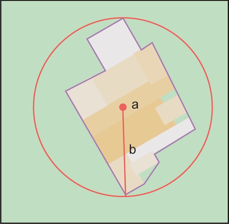
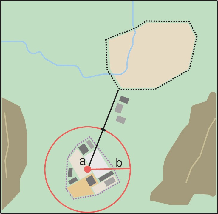
Offsets
Locality Type |
Calculation Steps |
|---|---|
An offset is a displacement from a reference location, usually used in conjunction with a heading to give a distance and direction from a feature. |
|
Step 1: Determine the feature boundaries using the method for Geographic Feature only (§2.1) and add a buffer that is the distance given in the locality description, and there is no need to account for the proximity of other features. Step 2: Determine the coordinates of the corrected center and the geographic radial. Offset Distance = 0. Distance Precision = precision with which the distance was recorded in the locality description. |
|
Step 1: Determine the feature boundaries using the appropriate method for Geographic Feature only (§2.1). Account for the offset at a heading using other information in the record, or until reaching the proximity of another similar feature, whichever is nearer the original feature. Call this the "extended feature". Step 2: Determine and use the coordinates and geographic radial of the extended feature. |
|
The locality consists of a reference feature to start from and a distance to travel along a path. The path can be Narrow (§2.2.3.1) or Wide (§2.2.3.2). At times there may be Multiple Possible Paths (§2.2.3.3). Please reference the appropriate section for specific instructions. |
|
Step 1: Determine the boundary of the feature using the appropriate method for Geographic Feature only (§2.1). Step 2: Determine and use the coordinates of the corrected center and geographic radial of the estimated feature boundaries as the Input Latitude and Longitude. |
|
Step 1: Determine the starting feature using the appropriate method for Geographic Feature only (§2.1). Step 2: Determine and use the starting feature coordinates and the geographic radial. |
|
Step 1: Determine the starting feature using the appropriate method for Geographic Feature only (§2.1). Step 2: Determine and use the starting feature coordinates and the geographic radial. |
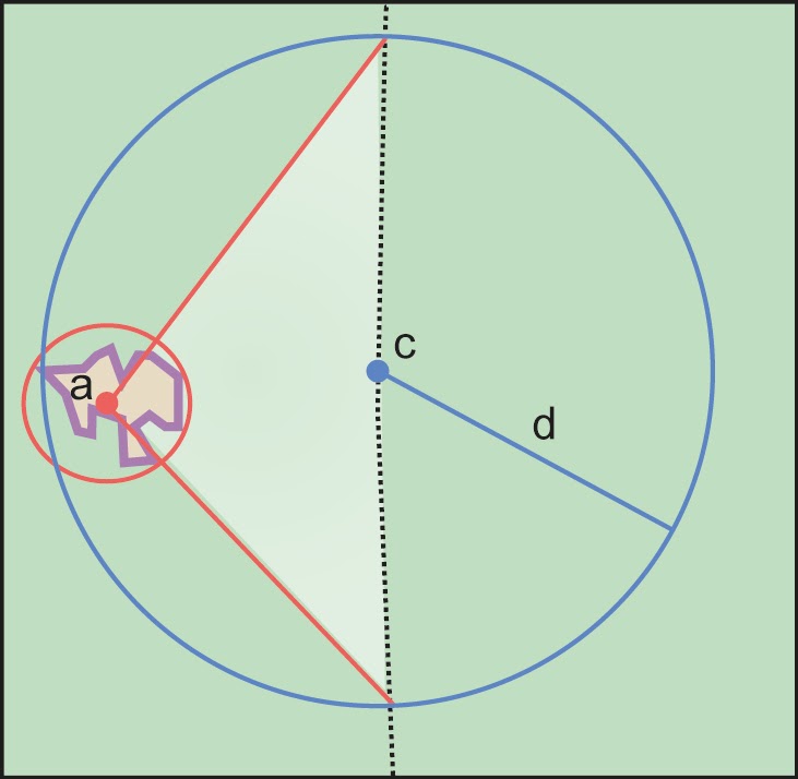
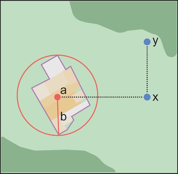
Coordinates
Locality Type |
Calculation Steps |
|---|---|
The locality consists of a point represented by latitude and longitude in one of various coordinate formats. |
|
Step 1: Use the coordinates in the format they were captured from a GPS or from the verbatim locality as the Input Latitude and Longitude. |
|
Although this is not technically a feature, the Geographic Feature only (§2.1) locality type in the Georeferencing Calculator (Wieczorek & Wieczorek 2020) includes all of the relevant parameters. Step 1: The Universal Transverse Mercator UTM coordinates must be converted to decimal degrees using a UTM to Latitude/Longitude conversion tool. The UTM Zone is required to do this. Step 2: Determine the geographic radial: If the UTM coordinates have 7 digits in the northing and 6 digits in the easting, the geographic radial is 0.707 m. For UTM coordinates with fewer digits of precision see Table 1 (§2.1.2). |
|
Step 1: Determine the coordinates of the grid cell as for a Feature – with Obvious Spatial Extent (§2.1.1). Use the coordinates for the corrected center of the named grid cell. Step 2: Determine the geographic radial. |
Difficult Localities
Locality Type |
Calculation Steps |
|---|---|
The locality is vague or presents other challenges. It is recommended to check the original catalogues, ledgers, field notes, specimen labels, etc. as a first step to resolve the vagaries. |
|
If some part of the locality description is in question, but there is locality information that is not in question, use the unquestioned part of the locality to determine the locality type and georeference following the appropriate method. If the entire locality is in question, do not georeference and document in georeferenceRemarks the reason for not georeferencing (e.g. "locality in question"). |
|
The cited locality cannot be found. Reasons may include: Do not georeference these localities. Document in georeferenceRemarks (e.g. "locality cannot be found with available references"). |
|
Multiple related features: If there are multiple distinct nearby places with the same name and no further information to distinguish between the possibilities, treat the combination of them as the feature and follow the procedure for the appropriate locality type. Document in georeferenceRemarks. Multiple unrelated features: Do not georeference. Document in georeferenceRemarks (e.g. "there are multiple possible unrelated features matching the one in the locality description"). |
|
The locality description contains irreconcilable inconsistencies – assertions that can not all be simultaneously true. Do not georeference. Document in georeferenceRemarks. |
|
The locality is associated with a captive animal, a cultivated plant or an event from some other non-natural occurrence. The locality cited is often that of a zoo, aquarium, or botanical garden. Georeference the locality normally based on the locality type and feature. Document the nature of the provenance using the term degreeOfEstablishment. |
Appendix B: Methods to Find the Corrected Center and Geographic Radial
Introduction
Sometimes determining the corrected center and geographic radial of a feature can be difficult to do "by eye." It usually requires repeated trial and error moving and adjusting the radius of circles to narrow in on the final result. Here we share some simple methods to aid in finding the corrected center and geographic radial based on the geometric shape of the feature of interest.
Linear Feature
Method |
|
|---|---|
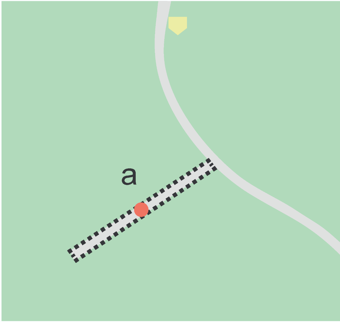
|
Step 1: Find the midpoint of the segment a that joins the two most distant points of the geometry (solid line). |
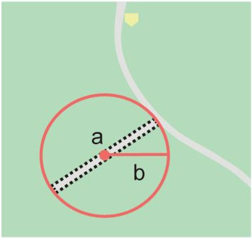
|
Step 2: The midpoint is the corrected center a. The geographic radial is the distance from there to either end of the line segment b. |
Elongate Convex Feature
Method |
|
|---|---|
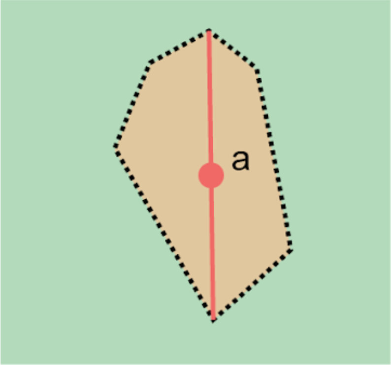
|
Step 1: Find the midpoint of the segment a that joins the two most distant points of the geometry (solid line). |
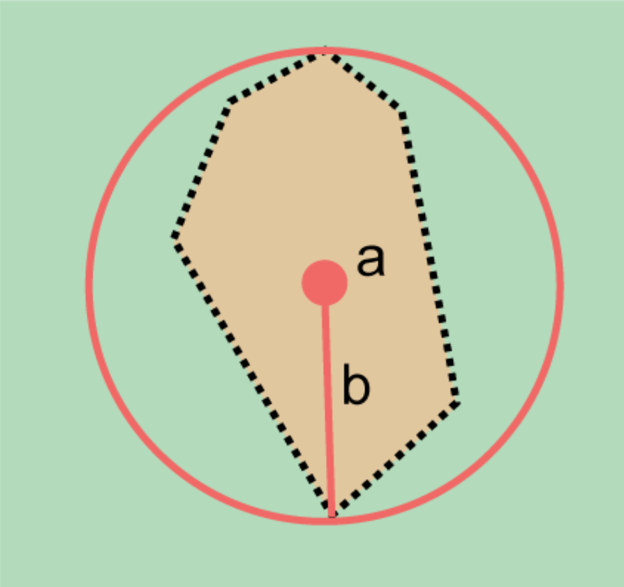
|
Step 2: If the midpoint is within or on the boundary of the geometry and there is no point within the geometry that is further away than the two extreme points of the chosen segment (which one can determine by eye, with a ruler or with a tool to make a circle), then the midpoint is already the corrected center a, with geographic radial b. |
Not Obviously Elongate Convex Feature
Method |
|
|---|---|
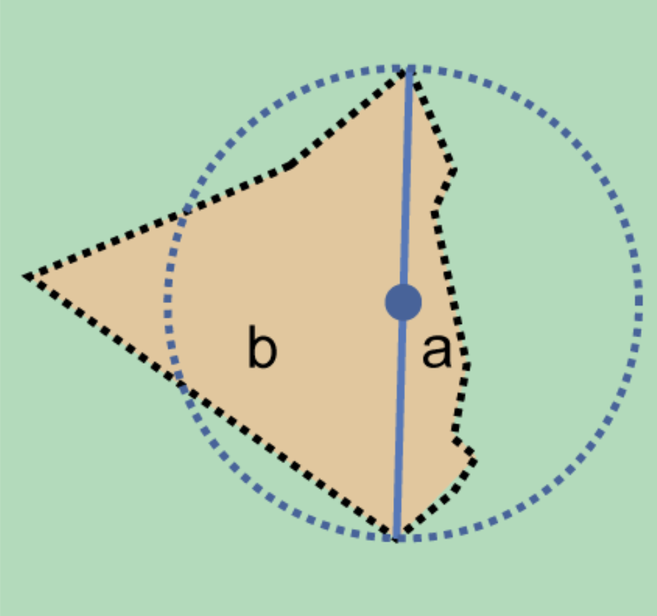
|
Step 1: Find the midpoint a of the segment that joins the two most distant points of the geometry (solid line). Draw a circle with center at the midpoint and diameter up to the two ends of the segment (dotted circle). |
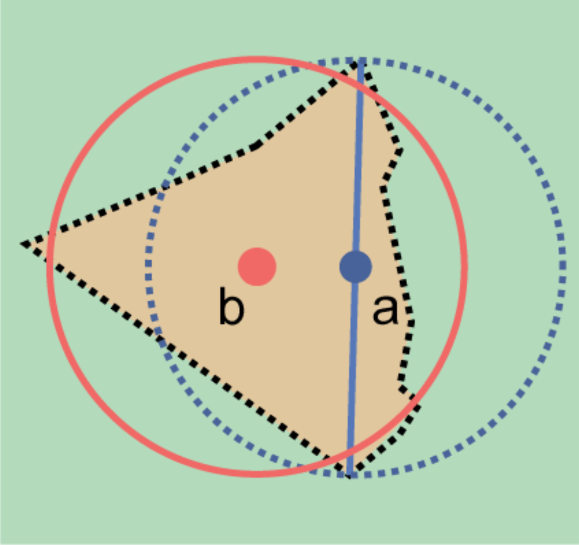
|
Step 2: If any point of the geometry falls outside the circle, move the circle so that the farthest spaced vertices of the geometry are equally far outside the new circle (solid circle, with center b). |
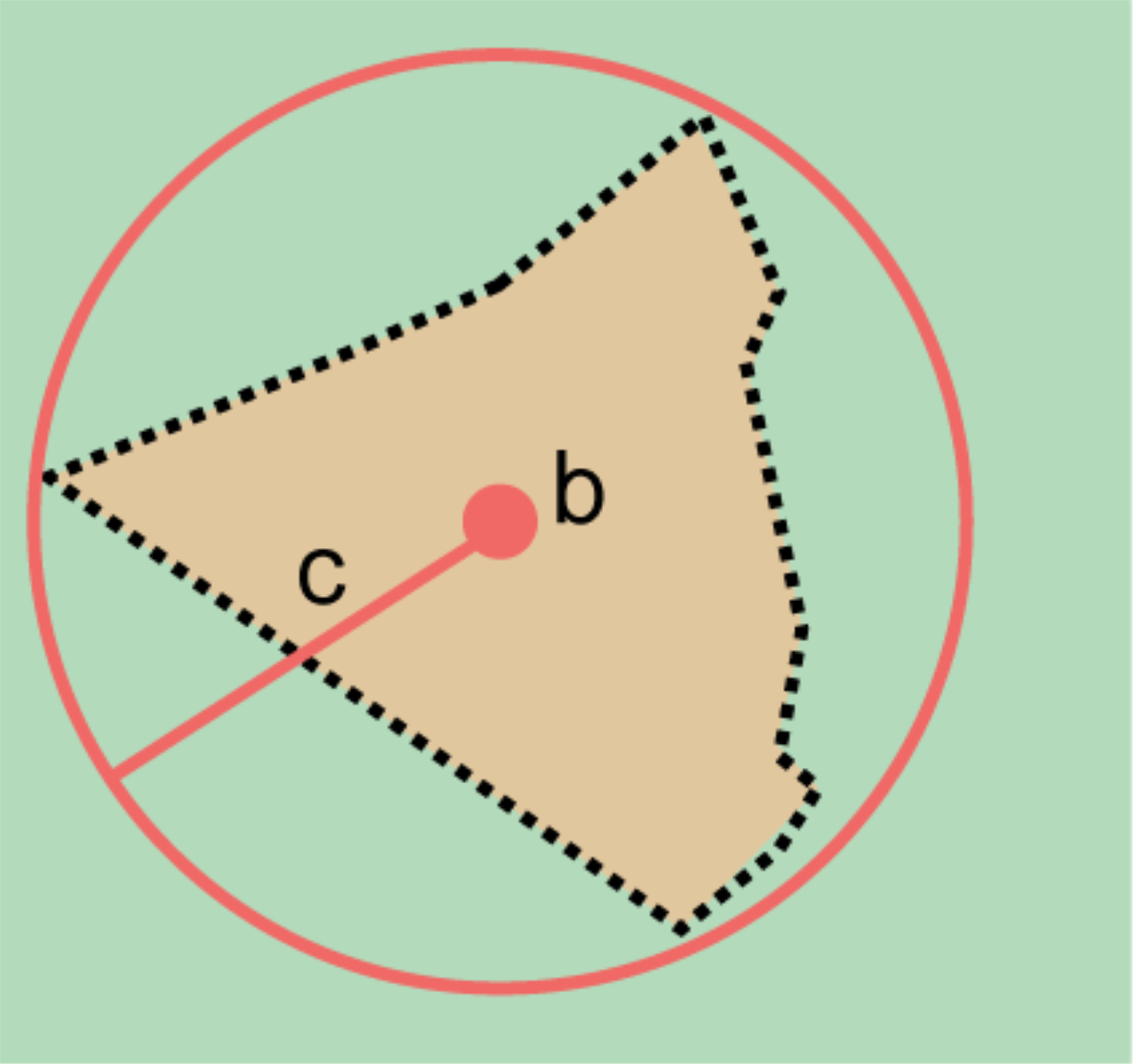
|
Step 3: Increase the radius of the circle, without moving the center, to just include the most distant points of the geometry. The center of this circle b is the corrected center with geographic radial c. |
Simple Concave Feature (center within the feature)
Method |
|
|---|---|
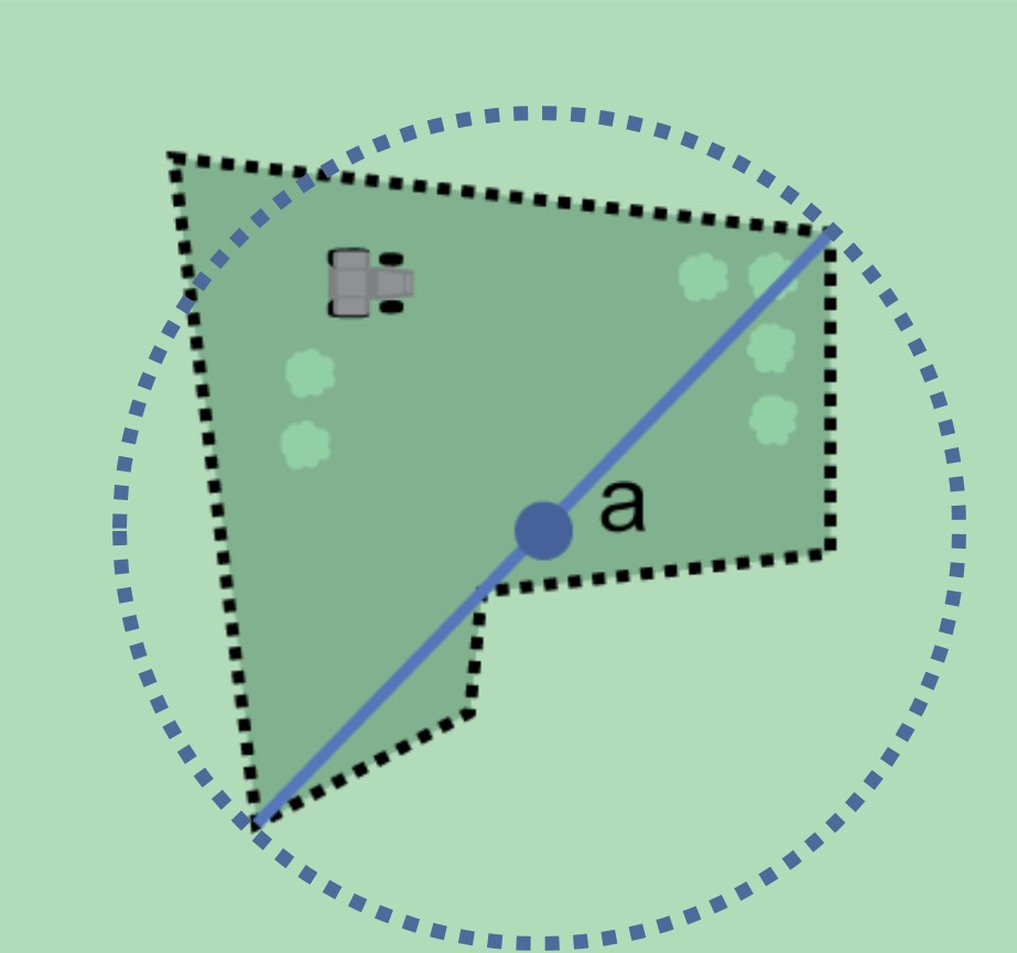
|
Step 1: Find the midpoint a of the segment that joins the two most distant points of the geometry (solid line). Draw a circle with center at the midpoint and diameter up to the two ends of the segment (dotted circle). |
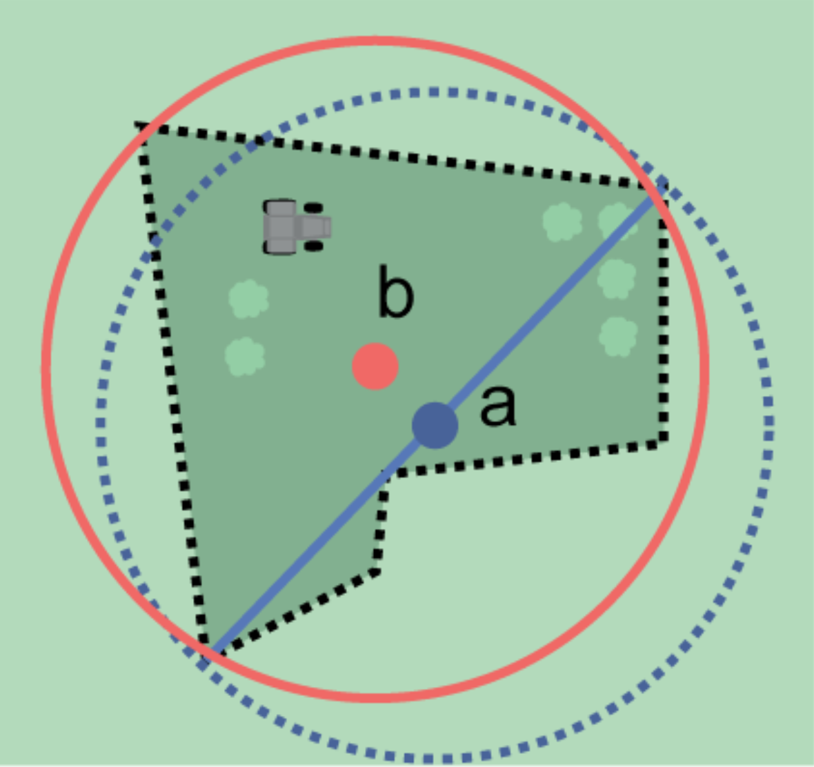
|
Step 2: If any point of the geometry falls outside the circle, move the circle so that the three farthest spaced vertices of the geometry are equally far outside the new circle (solid circle with center b). |
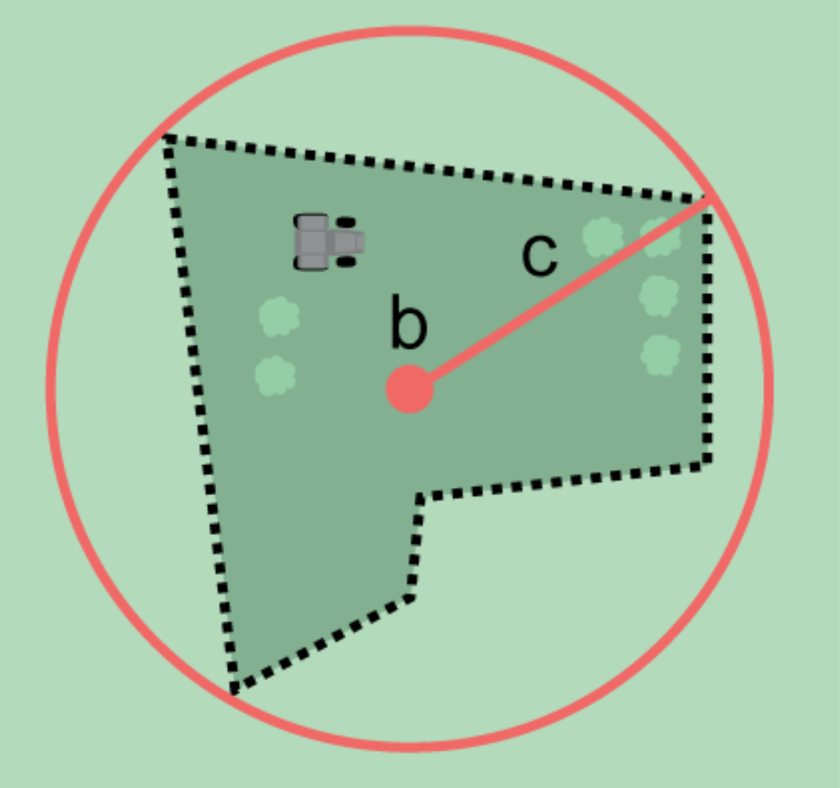
|
Step 3: Increase the radius of the circle, without moving the center, to just include the most distant points of the geometry. The center of this circle b is the corrected center with geographic radial c. |
Complex Concave Feature (center outside the feature)
Method |
|
|---|---|
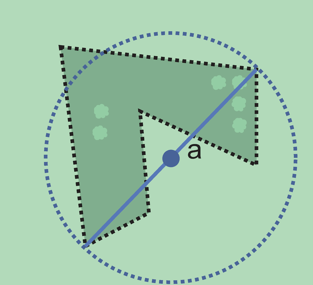
|
Step 1: Find the midpoint a of the segment that joins the two most distant points of the geometry (solid line). Draw a circle with center at the midpoint and diameter up to the two ends of the segment (dotted circle). |
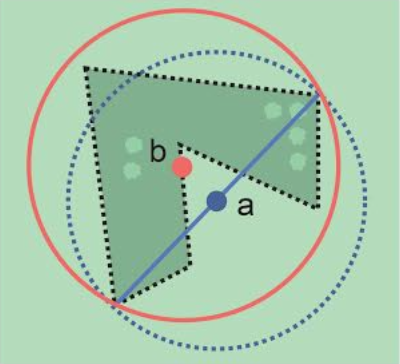
|
Step 2: Move the circle so that the center falls on the border of the geometry and the vertices that are farthest spaced are equally far outside the new circle (solid circle with center b). |
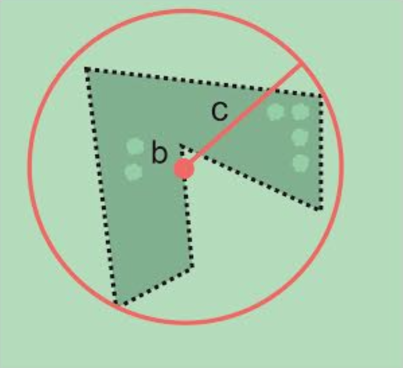
|
Step 3: Increase the radius of the circle, without moving the center to just include the most distant points of the geometry. The center of this circle b is the corrected center with geographic radial c. |
Curvilinear Feature
Method |
|
|---|---|
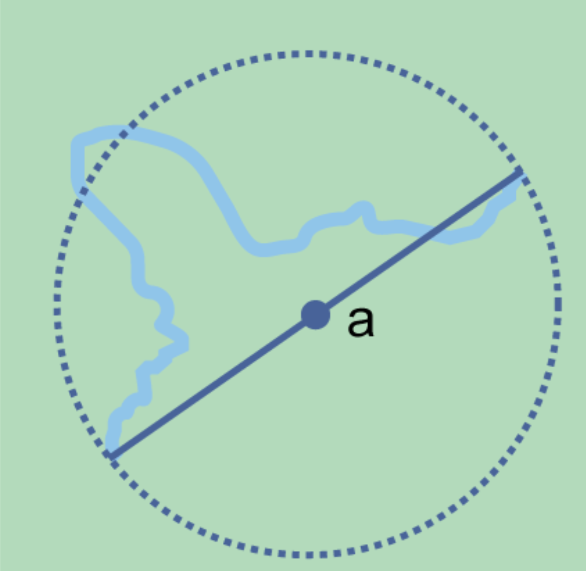
|
Step 1: Find the midpoint a of the segment that joins the two most distant points of the geometry (solid line). Draw a circle with center at the midpoint and diameter up to the two ends of the segment (dotted circle). |
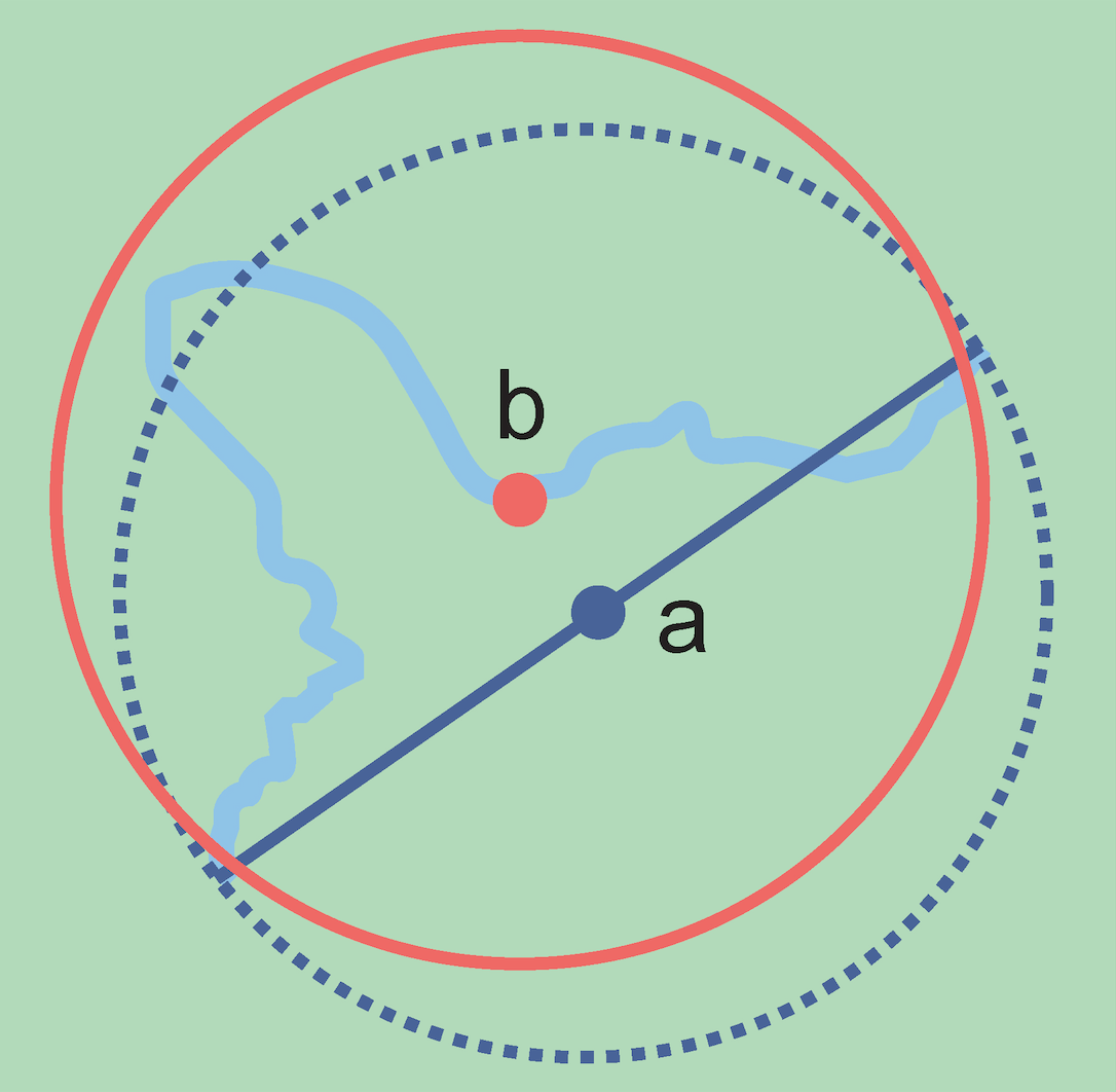
|
Step 2: Move the circle so that the center falls on the border of the geometry and the vertices farthest from there are equally far outside the new circle (solid circle with center b). |
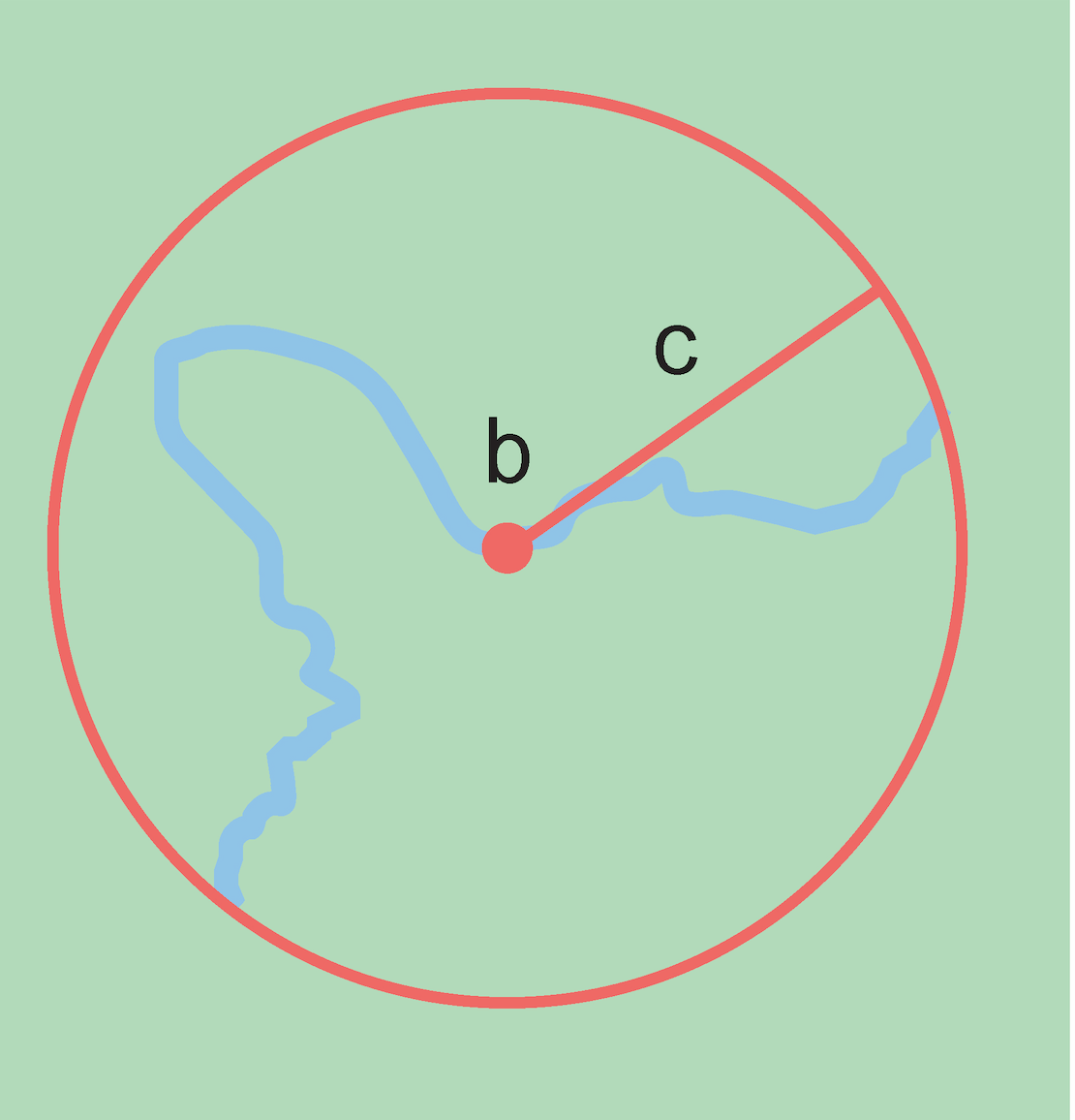
|
Step 3: Increase the radius of the circle, without moving the center to just include the most distant points of the geometry. The center of this circle b is the corrected center with geographic radial c. |